Nitrogen cycling

In this exercise you will observe the fate of fertiliser nitrogen in a fallow situation: Urea to ammonium to nitrate and the loss of soil nitrate via denitrification.

This simulation will introduce us to editing a simple Manager rule and to more advanced features of graphing simulation results. Firstly we need to set up our weather and soil data. The simulation is on silt soil in the Bhola region in Southern Bangladesh.

Start with a new simulation based on Continuous Wheat
Change simulation name to Silt Fertilised
Save the file as N Fallow.apsim (C:\Apsim_workshop\N fallow.apsim)
Choose a weather file for Bhola (c:\Apsim_workshop\met_files\Bhola_1998-07.met)
Set the clock starting date: 1/1/2001 Ending date: 31/12/2001
Add a soil to the field node (North Joynags-06 No673)
From Soils toolbox, find and drag a “Southern Bangladesh, Bhola district Silt, (Wheat PAWC = 138.5 mm, 1.5m)” soil file (“Soils” –> Bangladesh –> Southern Bangladesh –> Bhola –> “Silt (North Joynags-06 No673)”) onto the field node of the simulation tree. Remove the existing soil after the addition of the new soil. Rename the soil to something short like “Silt”. If you like you can also reorder the soil component so it comes straight under the paddock. (Hint: Highlight your soil and use the Ctrl & up arrow to move a node up the tree)
Set the Starting water to 50% full, evenly distributed.
At the Initial nitrogen node, set the starting NO3 to 10 kg/ha (i.e. 6 and 4 in the 0-20 and 20-200 layers) and starting NH4 to 5 kg/ha (i.e. 4 and 1 in the two layers)
Set the initial surface organic matter to 2000 kg/ha wheat residues.
Remove the wheat component from the paddock, and all manager rules from the manager folder.
Drag a Fertilise on fixed date to your Manager component. (“Standard toolbox” -> “Management” -> “Manager (common tasks)” )
Select Fertilise on a fixed date to edit:
Enter fertiliser date: 15-Jan.
Don’t add fertiliser if N in top 2 layers exceeds: 1000.
Module used to apply fertiliser: fertiliser.
Amount of fertiliser to apply: 100.urea_N.
Make sure your simulation contains a Fertiliser component in your paddock. Even though it doesn’t have any changeable properties it is still necessary when fertiliser is to be applied.
Select Outputfile Variables.

Add the following variables to report:

Component	Variable name
Clock	dd/mm/yyyy as Date
	Year
	Day
Met	Rain
Soil (Silt)	dlayer The thickness (in mm) of each soil layer
	esw Extractable Soil Water (mm)
	drain Drainage (mm)
	NO3() as NO3_Total Nitrate Nitrogen, summed over profile, aliased to NO3Total. (the as keyword creates an alias)
	NH4() as NH4_Total Ammonium Nitrogen, summed over profile, aliased to NH4Total
	UREA()
	DNIT()
	NO3 Nitrate Nitrogen, layered
	NH4 Ammonium Nitrogen, layered

Change reporting frequency (under Outputfile) to end_day.
Run the simulation
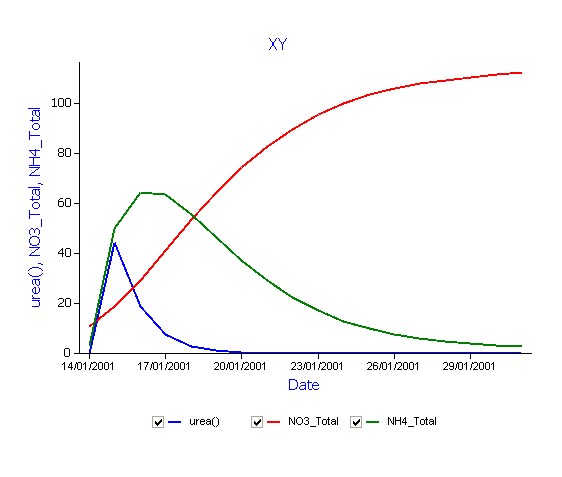
Create a graph of date vs urea, total ammonium and total nitrate. Drag an XY graph component onto the simulation. On the Plot node set “Point type” to None and leave “Type” as Solid line.

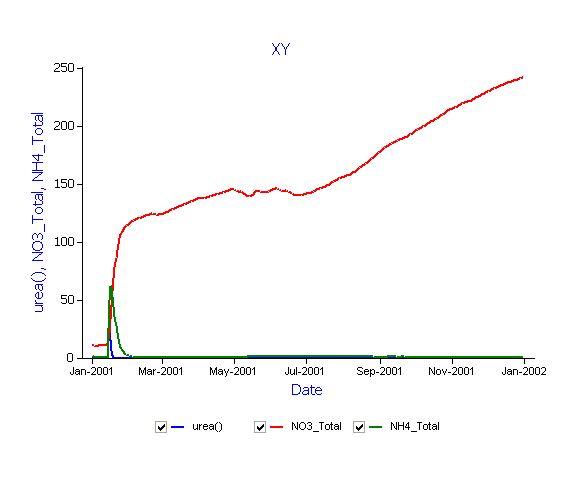
Question: Why does the above graph look the way it does?

Illustrating the extent and conditions required for denitrification losses

Create a new chart of Date vs Rain, DNIT (right hand axis), ESW and NO3_Total.

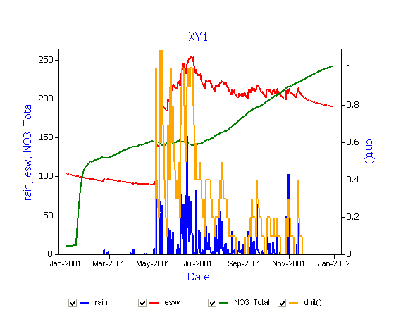
From this chart you can see that some nitrogen is lost via denitrification when large amounts of nitrate is available in saturated soil conditions. But why do you think the level of denitrification is so low (0.1 kgN/ha/day) in this case?

Exploring vertical movement of nitrate, after fertilisation, through the soil profile

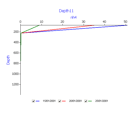
Let’s look at the distribution of nitrate through the soil profile at the day fertiliser is applied and then at 1, 3 and 5 months after fertilisation.

Create a depth graph (from the graph toolbox), and expand all the sub-nodes. Go to the depth node, and select (so that they show a tick mark) the dates 15/01/2001, 15/02/2001, 15/4/2001 and 15/5/2001. Go to the Plot node and select NO3 as the X variables. Leave the Y variable as “Depth”. Select the top graph node (“Depth”).Depth plots can only be done when the simulation has “dlayer” in the output file along with at least one other layered variable. This is why we included no3 and nh4 as layered variables in the output file and not just the summed variables for NO3() and NO4(). (Hint: adding () to an array variable like “NO3” to form “NO3()” will sum the nitrate values from all the soil layers)

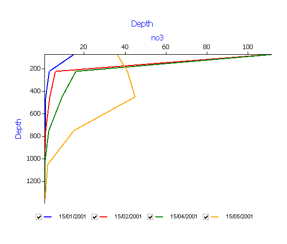
From this chart you can see the change (on the X axis) in the distribution of nitrate (NO3) in the soil profile (Y axis) over time in response to the addition of urea fertiliser and leaching processes at the start of the wet season. (The default title “Depth” can be changed to something more suitable ie. Change in soil NO3 over time

Question: Why is there little change before the 15th of May?

Repeat the steps above and create another graph this time selecting NH4.

Notes:

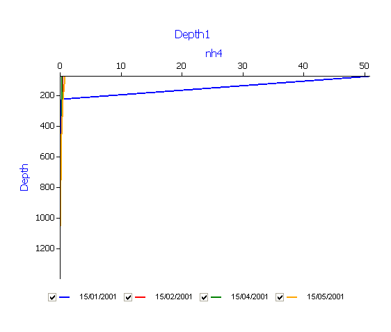
Question: What has happened to the NH4? Try changing the dates to look at NH4 at 1, 5 and 10 days after fertiliser has been applied.

From this chart you can see the change in the distribution of NH4 in the profile occurs very rapidly over the course of a few days. NH4 is converted to NO3.

Additional exercise: Try creating another simulation with clock set between 14/01/2001 and 31/01/2001. Create a time series graph of urea(), NO3_total and NH4_total in the profile over a period of 15 days after fertiliser is applied. Would the simulated process be the same if the fertiliser was applied in the middle of the wet season (August)?

Movement of Nitrogen between Organic Matter Pools

In this exercise we track the movement of nitrogen in fresh organic matter into soil microbial biomass and further into mineral nitrogen. We shall compare the flows in these processes for incorporation of two types of residues – wheat and cowpea.

Make a copy of the Silt fertilised simulation by dragging to the top node in the tree (Simulations)
Delete all the XY and Depth graphs. – This setup already includes wheat residues on the surface at 2000 kg/ha and C:N ratio of 80
Change starting NO3-N to 60 kg/ha (36 and 24 in each of the 2 layers), leaving NH4-N at 5 kg/ha
Remove Fertilise on fixed date from your paddock component
Drag Tillage on fixed date to the Manager folder in your ‘paddock’ component for this new simulation. (open “Standard toolbox” -> “Management” -> “Manager (common tasks)” )
Change the Tillage management parameters to: date = 15-Jan
Module used to apply the tillage = Surface Organic Matter
Tillage Type = user_defined
User defined depth of seedbed preparation = 100 (mm)
User defined fraction of surface residues to incorporate = 1.0
Change simulation name to Silt wheat residues incorp.
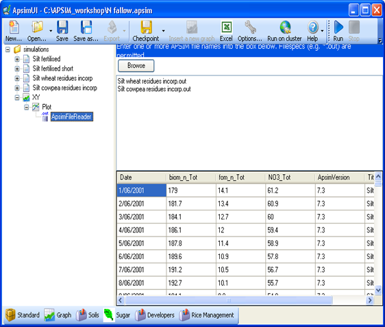
Choose these variables to report:

Component Variable name

Clock dd/mm/yyyy as Date

Soil (Silt) Biom_n() as biom_n_Tot

Fom_n() as fom_n_Tot

NO3() as no3_Tot
Create a copy of the Silt wheat residue incorp simulation and call it Sand cowpea residue incorp.
Change the initial surface residue parameters to 2000 kg/ha of Cowpea (type) residue. Set the C:N ratio to 20. (Remember you may want to change the Organic Matter pool name to cowpea as well. Remember to reflect this change in Tillage on a fixed date – Module used to apply tillage)
Run the two simulations for residue incorporation.
Graph both residue incorporation simulations with fom_n_tot (left hand axis), no3_tot and biom_n_tot (right hand axis), and fom_n_tot. (Drag an XY graph onto the top node (simulations), open the ApsimReader node and point to the 2 output files)

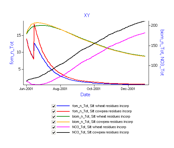
Inspect the change in fresh organic N in residues (fom_n) with time.

Note: There is a steep increase in the first few days when tillage incorporates the surface residues and this material is passed onto the soilN modules as FOM. Soil “fom_n” for legume is higher than for wheat residues reflecting the differences in N content of the 2 materials as determined by the C:N ratios input to the model.

Differences between wheat and legume dynamics in decomposition of FOM and its N content can be seen in the transfer of N into the microbial N pool (biom_n_tot), and the effects of this transfer on the net immobilisation/mineralisation of organic N from/to the soil nitrate pool. NO3 levels increase over time reflecting changes in fom_n and biom_n pools.

Question: Would these rates of change increase during the wetter and warmer months?