
Construct a factorial simulation in the User Interface
When running an Apsim simulation for analysis it is often necessary to run the model multiple times whilst changing a few key variables to get results that show a wider range of possible outcomes. An example of this would be to run the model with a range of Initial Water levels for a soil, a range of fertiliser rates, and a range of planting dates. For the best results, it would be necessary to run all possible combinations of the three.
The difficulty encountered in this situation is that each possible combination would require it’s own simulation in the simulations tree. Assuming 3 different planting dates, 3 different fertiliser levels and 3 different Initial Water values and you would need 27 unique simulations in the tree. If a change is required to the original simulation, it will also need to be repeated in 26 other simulations. With the use of linking, the number of changes could be reduced, unless it is a change to the structure – in which case the addition or removal of a component will result in changes still being necessary for every simulation.
Factorials attempt to solve this problem by allowing the user to define the variables to be replaced – called “Factors”, as well as the collection of values to replace them with – called “Levels”. It will then run the model with all possible combinations of those “Levels”. It will do this using only a single simulation.
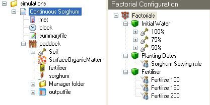
A Single Simulation with Factorials
Factor Nodes
A Factor node represents one or more “Factors”; each factor containing one or more “Level”. Each “Level” can be as simple as a single number, or as complex as an entire Soil component, depending on how the Factor node is configured. The factor node can be configured to behave in two possible ways; by replacing entire components, or by replacing individual variables within a component.
Component Replacement
The default behaviour of a factor node is to treat each of it’s child nodes as a “Level”. The level is applied to a simulation by completely replacing an entire component. It can also handle more complex components such as a Soil component. Selection of a component underneath the factor will enable the component to be displayed and editted as per usual.
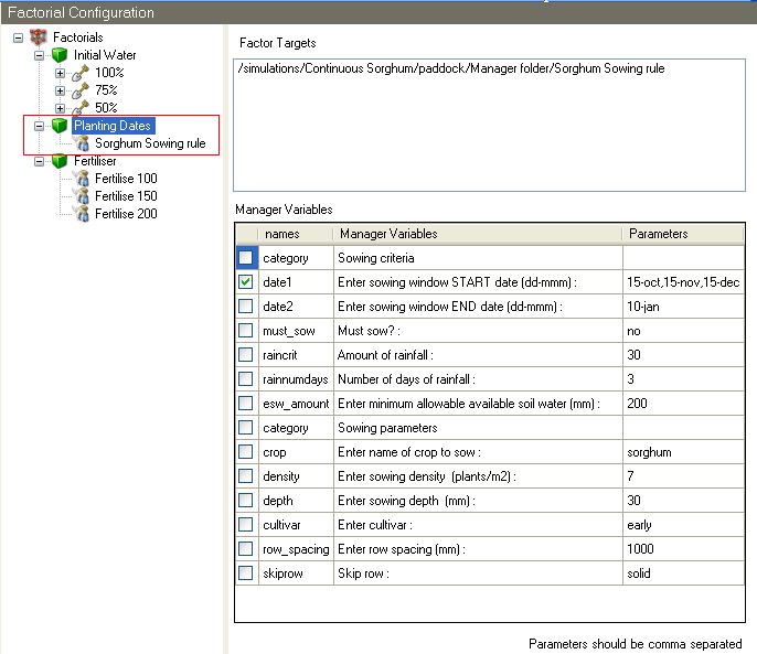
Variable Replacement
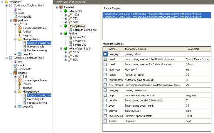
There are some components that store variables within their internal structure. If a factor node has a single child of one of these components, it will display a table of variables and their values. Each line in the table has a checkbox, which when checked will cause the variable to be treated as a factor. So it is possible for a factor node to have multiple factors by checking multiple rows in the table. The levels are defined in the Parameters column by comma separated values.
The component types that can be used this way are defined in factor.xml. At the time this documentation was written, a factor node could recognise 5 types of components which were defined like so:
<FactorVariables>
   <facvar>manager</facvar>
   <facvar>rule</facvar>
   <facvar>cropui</facvar>
   <facvar>sorghumconstants</facvar>
   <facvar>sorghumgenotype</facvar>
</FactorVariables>
The two sorghum components are a list of variables, each defined by a node named “property”. The name of the variable is contained in the “name” attribute (which allows spaces) and the value is again stored in the inner text property of the node. The factorial component again simply replaces the inner text property of the appropriate variable.
<SorghumConstants name="standard">
   <property name="crop_type">sorghum</property>
   <property name="default_crop_class">plant</property>
</SorghumConstants>
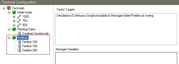
Targets
Each factor node has a list of one or more targets attached to it. Each target is the location of a component that will either be replaced, or updated depending on the type of factor node. When a target is selected in the list, the designated component will be highlighted in the selections tree. A target can be created by selecting the component in the simulations tree and dropping it onto the list of targets. This will add that component onto the list. A target is also added to the list automatically when dragging an item from the selections tree to be a level underneath a factor node.
Please note: At present, renaming a component within the targets path will cause the target to be invalid.
Targets can enable more complex scenarios to be configured. Using the initial example that used Initial Water, Fertiliser and Planting Date as variables, what would happen if a second simulation was added to model a different soil type at the same location. The simulation can be created by dragging the current simulation to the simulations folder, causing a copy to be made. A different soil needs to be added to the new simulation and the old one removed. The Initial Water factor will be invalid for the new simulation as it uses a different soil type – Note: the model won’t be able to determine that it is wrong. A new Initial Water factor based on the new soil type will need to be created.
Targets in Site 1:
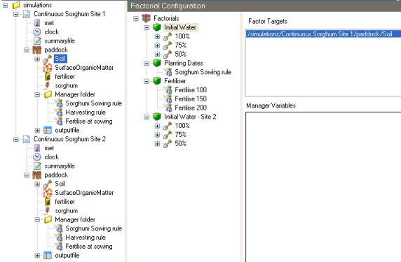
Targets in Site 2:
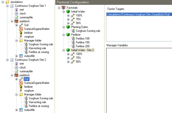
Both Simulations are Targets:
Targets Walkthrough
1. If renaming the new simulation, please do so before setting up the factors.
2. Right click on the factorials node and select Add Factor (rename it to “Initial Water Site 2”)
3. Select and drag the Soil component added to the new simulation onto the new factor.
4. Repeat step 3 twice more (there should be 3 Soil components under the new factor).
5. Expand the first soil node under the new factor and select the Initial water component
6. In the text box within the group titled “Specifying a fraction of maximum avaialble water”, make sure the value is 100.
7. Repeat steps 5 and 6 on the second soil node, but this time enter 75%.
8. Repeat steps 5 and 6 on the third soil node, but this time enter 50%.
9. Rename the soil nodes 100%, 75% and 50% respectively.
10. Select the factorials node, it should show two simulations, with a count at the end of each one. The first simulation should still be showing (27) – which is the number of simulations it will create and run. The new simulation should be showing (3). When the soil node was dragged to the new Initial Water factor, it automatically added the soil as a target to the Factors target list.
11. Select the Planting Dates factor node to display it’s list of Targets.
12. Add the Sorghum Sowing rule in the new simulation to the Targets list of the Planting Dates by selecting it and dragging it across to the Planting Dates Targets list.
13. Repeat this process using the Fertilise at sowing node in the new simulation and dragging it to the Targets list of the Fertiliser factor.
14. Select the factorials node and it should show 2 simulations with (27) each.
Current Limitations
At present it is difficult to model different locations using a single simulation through the use of factors. The factorial component will iterate through all possible combinations of factors that have targets to a given simulation. Using the walkthrough example, if the soil component is added to the targets list of “Initial Water Site 2”, it will result in 81 runs instead of 54. This number can be calculated by 3 (Inital Water) x 3 (Planting Dates) x 3 (Fertiliser) x 3 (Initial Water Site 2). It would have been possible to add 3 new soils to the existing Initial Water, which would have resulted in 6x3x3, or 54 runs as was desired. When dealing with different locations though, there is a 2nd factor that will normally need to be changed between sites – rainfall data (which is defined within the met component). Adding a factor node for met files with 2 Levels, each representing a different location will result in 108 simulations (6x3x3x2). It would combine both met files, with both soil types, which was not desired. It would be necessary to create 2 simulations to provide a valid solution.
Future Development
Having to create a separate simulation for each location defeats the initial goal of reducing the time required to create and maintain complex combinations.
Complex Factors
Complex factors will allow multiple components to be attached to a single factor eg: a met file and soil component. To provide a solution to the last example, 6 complex factors could be created, each containing a soil and a met file, resulting in 54 runs (6x3x3). It would also be able to handle multiple met files (climate forecasting) by adding more complex factors to the list.
Factor Hierarchy
Complex factors will provide a solution to multiple locations that all use the same set of variables. When dealing with multiple locations though, not all of the variables might be relevant to all locations. Sowing dates can vary between locations, which can be modelled using the whole range of possible dates, but results in extra simulations being run and then needing to be removed from the results as they are invalid. In order to do this, there needs to be a way to create separation between the factors, while still being able to use those factors that are common to all situations. This result can be achieved through the use of a hierarchial structure that allows both separation via folders, and inheritance via parent nodes. The easiest way to explain this is to look at an example image.
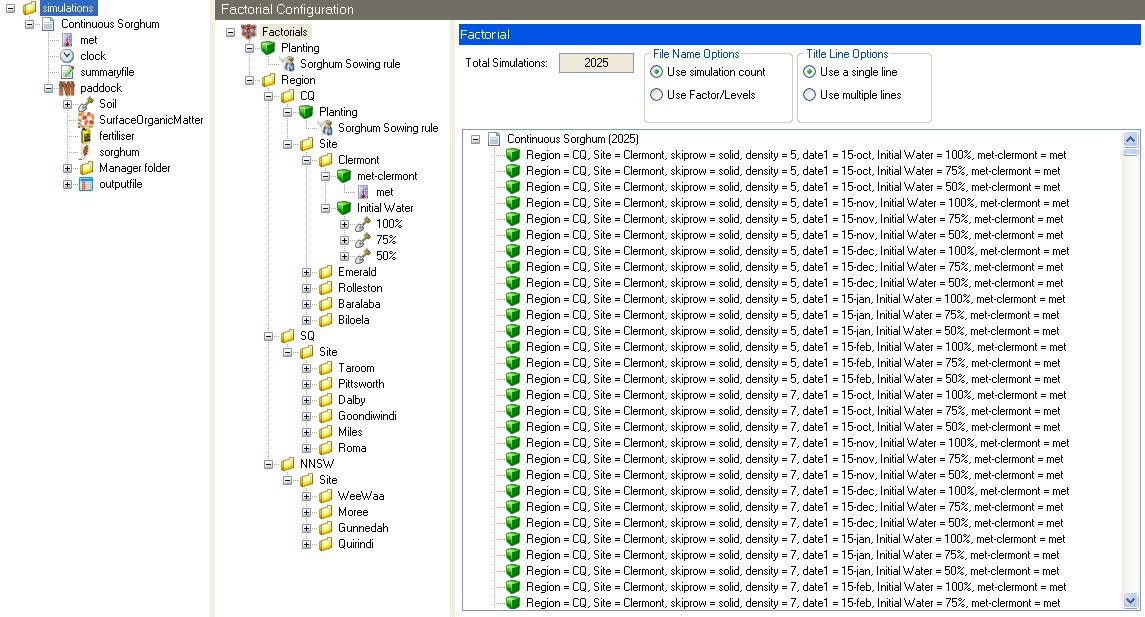
The following walk through explains how this structure was created.
1. Start with the Continuous Sorghum Example project, and enable Factorials
2. Add those factors that will be common to all scenarios. Use a factor with a manager component to define planting dates (inheritance will be used to override the base factor), density and skip row status.
3. Add a Factor folder and rename it to “Region” which will represent a factor.
4. Add 3 Level folders to the “Region” factor called “CQ”, “SQ”, “NNSW” respectively
5. Add a Factor folder to each region called “Site”
6. Add a number of Level Folders to each “Site” factor to represent different sites in that region.
7. Each site should have a “met” factor which will have a met component pointing to that particular sites met data
8. Each site should have a “Initial Water” factor, which will contain 3 copies of the same soil, except the Initial Water value will be different for each one (100%, 75%, 50%).
9. CQ has different planting dates to the other two regions, so the Planting factor is copied to the CQ factor folder.
10. Change the planting dates for the CQ Planting factor, and uncheck the density and skiprow rows. This will overwrite the Planting dates, but not the density and skiprow values.
11. The first line of output should now be “Region=CQ,Site=Clermont,date1=15-oct,density=5,skiprow=solid,met=Clermont Met,Initial Water=100%