
Fallow Water Balance
In this exercise you will explore the major elements of interest in soil water balance during a fallow – soil water storage, drainage, runoff, and evaporation. Changes will be examined over a one year period in the Bhola district of southern Bangladesh. The examples assume you have read and walked through the document: Introduction to APSIM UI
It is suggested that you first create a custom worshop directory: c:\Apsim_workshop for saving the simulations generated from these exercises.
Create a sub-directory: c:\Apsim_workshop\met_files to store your APSIM weather files.
Note: You may want to copy the two weather files that are required to complete these exercises, Bhola_1998-07.met and Dinajpur.met into your workshop met file directory from: C:\Program Files\Apsim73\Examples\MetFiles.
- Create a new simulation using a blank simulation as a starting point
- Choose a weather file for Bhola (Bhola_1998-07.met)
Note: Weather files can be found in the directory: C:\Program Files\Apsim73\Examples\MetFiles or in c:\Apsim_workshop\met_files. - Starting date: 1/1/2001 Ending date: 31/12/2001
- Rename paddock node to field
- Add a soil to the field node. A suitable soil characterised for the Bhola region would be : “North Joynags-06 No673”.
- From Soils toolbox, find and drag a “Southern Bangladesh, Bhola district Silt, (Wheat PAWC = 138.5 mm, 1.5m)” soil description onto the ‘field’ node of the simulation tree, (located under Soils –> Bangladesh –> Southern Bangladesh –> Bhola –> Silt (North Joynags-06 No673)). Rename the soil to something shorter like Silt.
- Set the starting water to 100% full – filled from the top. (expand the soil branch to see InitWater – i.e. click the “+” next to Silt)
- At the Initial nitrogen node, set the starting NO3 to 10 kg/ha (i.e. 6 and 4 in the 0-20 and 20-200 layers) and starting NH4 to 5 kg/ha (i.e. 4 and 1 in the two layers)
- Add Surface organic Matter to the field:
From Standard Toolbox – Soil related, drag a Surface Organic Matter component onto the field node - Check that the default initial OM pool name is rice_stubble and OM type is rice and the mass is 0 kg/ha. (at “surface Organic matter” node)
- From the standard Toolbox, drag a Outputfile onto the field node
- Select the outputfile’s Variables subcomponent. Choose these variables to report:
Component Variable name Clock dd/mm/yyyy as Date Year Day Met Rain Silt ESW – Extractable soil water (mm) ES – Evaporation Runoff DRAIN – Drainage NO3 – summed over profile (Do this by putting () next to the name in the “Variable name” column) eg. no3() (click “?” button next to variable list for more info) DLT_N_MIN – N mineralised – summed over profile Surface organic matter SURFACEOM_WT – Weight of all surface organic materials. SURFACEOM_COVER – Fraction of ground covered by all surface organic materials. - Select the “Outputfile” Reporting Frequency subcomponent. Delete “daily”. Choose end_day reporting frequency for the output file. This can be found under the Clock component filter
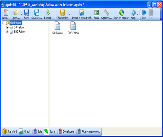
- Rename the simulation to something more meaningful: Silt Fallow
- Save the simulation file as “c:\Apsim_workshop\Fallow water balance.apsim”
- Run the simulation by pressing the “Run” button at the top of the ApsimUI.
- Create a graph of Date vs ESW.
Hint: To do this, click on the Graph Toolbox at the bottom of the window to open the toolbox. Then drag in an XY component onto the output file in your simulation. Click on the “+” symbol next to XY component to expand the node. Click on the Plot component. In the Plot window click on the X variables square to make sure the background of the square is pink. Now click on the “Date” column heading. It should appear in the list in the square. Now click on the Y variables square to make its background pink. Click on the esw column heading. It will be added to the Y variables square. To have a clean line plotted with no points, under “Point type”, choose “None”. Now click on the XY component to view the graph. - Once you have created a chart it is possible to make modifications by adding new variables. It is also possible to mix the type of plots used on a graph. As an example, we will add rain as a bar chart on the Y2 axis. To do this, drag “plot” onto the XY node to create a duplicate, plot1. At plot1, remove esw and add rain as the y variable. To make the “rain” appear on the right hand axis, click rain in the square to highlight it, then “right” mouse click on it again. In the popup menu click on “Right Hand Axis”. Select “bar” chart from “type” drop_down menu. Select XY node to see the line and bar chart combination.
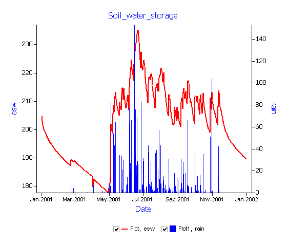
- Rename the XY graph node to ‘Soil_water_storage’
The graph should show the ESW (in mm) increasing with day of year. The sudden increases are due to rainfall events and the declines to evaporation and drainage loss. The distribution of daily rainfall amounts helps see this more clearly.
 Note: You can also examine other components of the simulated soil water balance.
 - Drag Soil_water_storage to the outputfile node to make a copy of this graphics node. Rename the copy to Runoff_drainage
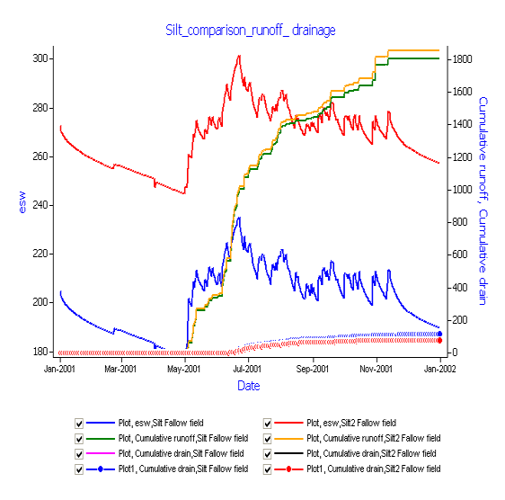
- At the Plot1 node underneath the ‘Runoff_drainage’ graph, remove rain from the Y variables box. Add runoff and drain to the Y variable box. Put both on the right hand axis (right click on the variable) to create a plot similar to the below figure.
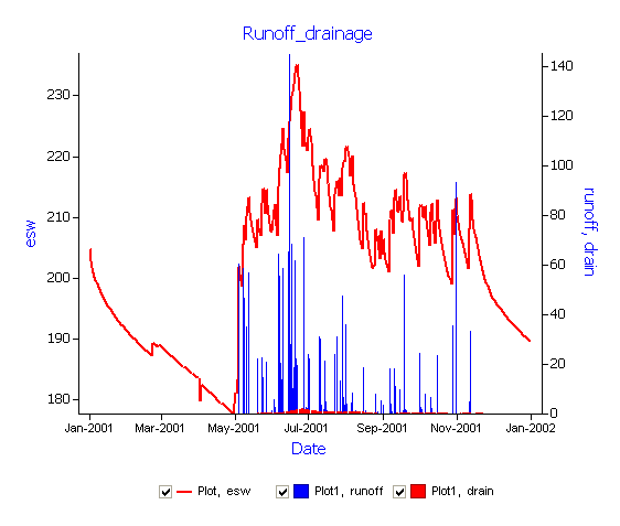
Runoff occurs from the start of the monsoon season early in May-June, continuing through the wet season till Nov-Dec. Drainage begins sometime after the first runoff, once the soil profile is near full. (Remember, PAWC for wheat in this soil is 138.5 mm, so the profile is mostly in a saturated state whenever esw is above this limit).
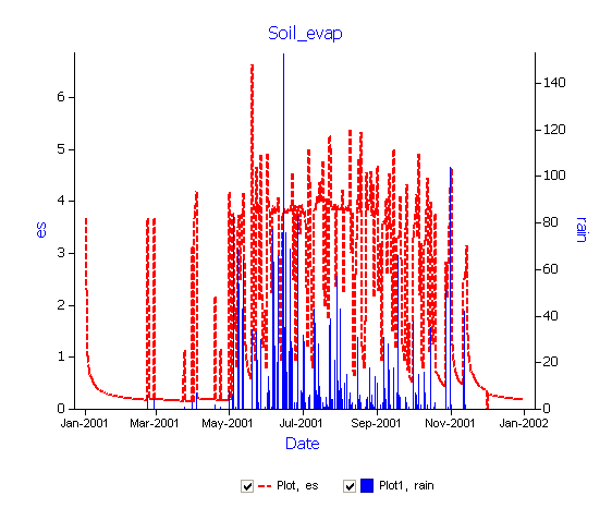
Additional exercise: You could also make a plot of soil evaporation. See if you can do this for yourself.
The effect of soil type on the water balance.
Runoff, es and drainage are affected by weather and soil water storage capacity. This simulation will add an additional soil and compare runoff from both soil types. The user interface still contains all the specifications provided for the previous simulation.
If you drag the Silt Fallow node in the Simulation Tree to the top node Simulations, a copy of it will be made and your file will then have 2 simulations in it.
This second simulation can then be modified to add the characteristics of a second silt soil with higher water holding capacity.
- From Soils toolbox, find and drag the Bangladesh -> Southern Bangladesh -> Patuakhali district -> “Silt (Shially-09 No783)” soil onto the paddock in the simulation tree and then remove the old soil (Hint: highligh the soil to delete and press the “Delete” key. It is important you drag in a new soil BEFORE you delete the old one, otherwise the simulation will lose all your soil reporting variables. Also remember to rename your soil to something shorter – eg Silt_2
- Since now we have a new soil we will need to go and set the initial soil water (InitWater) to 100% filled from top and initial soil nitrogen (Initial nitrogen) to NO3 to 10 kg/ha and NH4 to 5 kg/ha, as before. When you delete soils you also delete the initial soil water conditions and initial soil nitrogen conditions so these will need to be set similar to the conditions of the “Silt” soil.
- Rename the simulation to “Silt2 Fallow”.
- Save the simulations. (C:\Apsim_workshop\)
- Run APSIM for the Silt2 soil simulation.
- Graph both the output files by dragging an XY graph onto the top node Simulations in the simulation tree. By placing the XY graph under the “Simulations node”, all output files in the simulation area will be available for plotting – in this case, the Silt and Silt2 outputs.
- Create a graph of date vs esw and runoff(cumulative, right hand axis). To make the runoff cumulative, it is the same procedure as to make the rain appear on the right hand axis. Only select “Cumulative” from the popup menu instead of “Right Hand Axis”. Set “Point Type” to None.
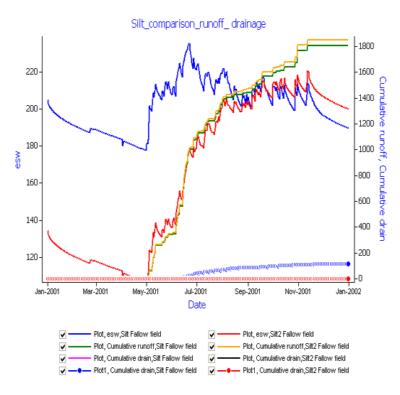
The figure below includes a plot of drainage for the 2 soils. See if you can also add ‘drain’ as shown above to your esw-runoff plot. (Hint: create a plot1, do cumulative and right hand axis and choose “circles” under Point Type)
The silt2 soil has only slightly higher runoff than the silt soil for all simulated events. Cumulative runoff for both is similar at over 1800mm. Is this what you might expect, given the PAWC of 33mm and the same rainfall and 100% full profiles as starting conditions? What can be seen from the accumulated drainage? Would runoff and drainage be the same if the initial PAWC for silt2 at the start had been different? (ie. Silt2 InitWater = 50%)
Notes:
Notes:
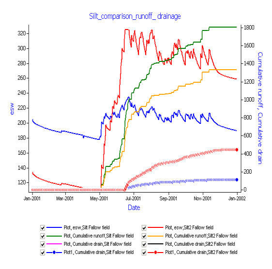
Additional exercise: explore the effect of changing curve number on the water balance. eg. for the silt2 soil, keep previous initial Plant Available Water Content (PAWC) settings at 50% (Silt2) and change curve number from 94 to 84 in the Soilwat node. What is the effect on accumulated runoff and drainage?
Changes to the water balance by ponding water on the surface.
In the previous exercises we have investigated the APSIM water balance on free draining soils in accumulating stored soil water and in simulating effects of runoff, drainage and soil evaporation. The soil specified in the previous examples reflect a typical soil in a natural (cultivated or uncultivated) state unaffected by (farmer) imposed physical constraints to the flow of water in the landscape. Rice production particularly during the wetter months of the monsoon is grown under paddy conditions. The natural structure of the soil surface has been modified (puddled) to reduce drainage and bunding (ponding) imposed to reduce runoff. These conditions therefore require some change to parameters in APSIM to simulate the effect of ponded water above the soil surface. The following exercise will use the ‘max_pond’ parameter to enable ponding of surface water and modify ‘KS’ (hydraulic conductivity) values for each soil layer to restrict the rate of vertical drainage.
- Drag Pond_depth on to the Manager Folder from “Rice Management Toolbox” -> “Rice” -> “Manager (Pond_depth)”
- Change properties to:
Name of your soil module: Silt
Start date for ponding: 1-Jun (Start of wet season – bunds constructed)
End date for ponding: 30-Oct (Crop maturing – open bunds)
Maximum depth of pond: 150
Minimum depth of pond: 0
Enable irrigation : No (set to No irrigation for the momemt)
Start date for irrigation: 1-Jul
End date for irrigation: 30-Oct
Maximum number of irriagtions allowed: 0 - Edit your soil file properties – Water – KS. (hydraulic conductivity in mm/day)to:
Component Variable name Depth KS 0-15 1.0 15-30 1.0 30-60 24.0 60-90 24.0 90-120 24.0 120-150 24.0 - Add additional report variables:
Component Variable name Met rain Soil DUL(1) sw(1) no3() drain runoff - Drag Irrigation on to the paddock field node in the “Silt Fallow Ponding” simulation from “Standard Toolbox” -> “Water Components (Irrigation)”
- Run APSIM for the Silt Fallow Ponding simulation.
- Create a graph of date vs DUL(1) and SW(1) (on Y axis) after deleting previous graphs. Rename this new graph to Ponding.
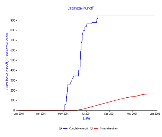
- Create a second graph by dragging Ponding onto your outputfile. Select runoff and drain (Cumulative) on the Y axis. Rename this graph Drainage-Runoff.
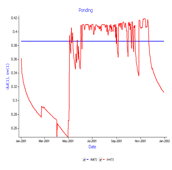
The Ponding graph shows the drained upper limit (DUL) of the first soil layer and volumetric soil water (sw(1)) in mm/mm for the first soil layer. Values above the DUL line indicate soil water over the drained upper limit and represent ponded water to a level as defined by “max_pond”. The Drainage-Runoff graph presents simulated values for cumulative runoff (in excess of water stored by “max_pond”) and cumulative drainage from the bottom of the profile as effected by “KS” input values.
Additional exercise: Explore the effect of changing ‘KS’ rates (mm/day) on the level of cumulative runoff and drainage.