Climate change projections
This exercise aims to explore the effects of climate change on maize cropping systems. Some background is in this PDF.
- Construct a long term maize simulation at Kakamega – use the Multiple season maize simulations as a guide (the examples below use the Maize_50N_10years simulation). For the analysis, we want to look at seasonal changes in rainfall, evaporation, transpiration and crop yields.
- Add the following lines to the tracker component:
Tracker variables sum of rain on start_of_day from sowing to now as RainSinceSowing sum of ep on end_of_day from sowing to now as Transp sum of es on end_of_day from sowing to now as SoilEvap - In the outputfile,we need to report the following variables:
Component Variable name Clock dd/mm/yyyy as Date Year Maize DaysAfterSowing Biomass Yield Manager DaysSinceSowing tracker RainSinceSowing SoilEvap Transp - Make a linked simulation and rename it to “Maize 350ppm”. There are several ways to make linked simulations:
a) right click and hold down on the source simulation and drag it to the top level (simulations) node. A popup menu appears when you let go, select the “Create Link Here” option.
b) Select the source simulation with the left mouse button, hold the keyboards <alt> key down, and drag it to the top level (simulations) node.
The advantage of linked simulations is that changes made to any component are made to all linked components. - Select the Maize 350ppm simulation (in blue).
- From the standard toolbox, drag an “ini” object from the “Structural” folder onto the maize component in the paddock. This will allow us to override the default “no CO2 response” maize parameterisation with one that has TE and N responses. Click the “Browse” button on the ini file component and point it at the file “Maize-7.3-CO2.xml” in the workshop files folder.
- Drag an “Empty Manager” component onto the manager folder of the simulation, and on its “init” tab, write the equation “CO2 = 350.0”. This will set the value of CO2 during the simulation to 350ppm.
- Run the simulation and verify that the results are identical to the first via a CDF plot.
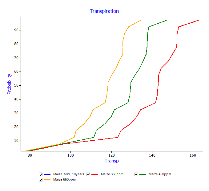
- Make two more linked simulations, change the ambient CO2 level to 450 and 550ppm respectively. Note changes in water use and crop yield. (NB. If you are using the Maize 350ppm simulation as the source, remember to unlink the manager node that sets ambient CO2.)
In crop rainfall and crop maturity times are identical in these simulations.
- Next we examine time to maturity (a function of temperature) – we begin by saving under a new name (Save As – Climate and Temperature.apsim). Remove all the linked simulations, ie. ones containing the “CO2” management tabs created above. Make new linked simulations for 2 temperature scenarios: +1, +2 degrees rise. Drag a “Climate Control” object from the Meteorological folder in the standard toolbox onto each of the linked simulations manager folders.
The “Climate control” component allows us to peturb both temperature by a constant amount, and rainfall by a percentage value. Once again, conduct a sensitivity experiment by increasing mean temperature by 1 degree intervals (ie. change in max = 0.5, change in min = 0.5):
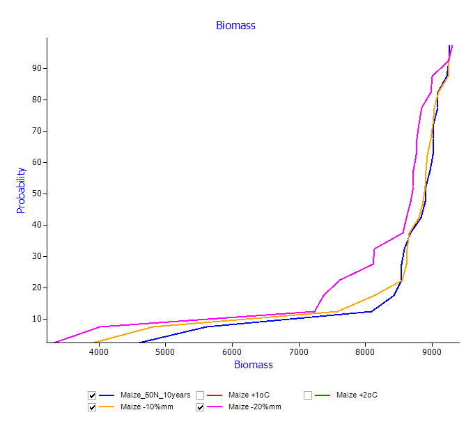
- Rainfall changes by -10, and -20 %age values:
Stochastic Weather generators and APSIM
The use of stochastic weather generators is not as simple – firstly met data is parameterised, the paramaterised generator is set to work making arbitrarily long weather sequences, and finally the systems model is run with each of these weather sequences. APSIM doesn’t include a weather generator – instead relying on the user to prepare met files with one of the commonly available programs such as LARS-WG, or Weatherman (included in DSSAT).
Using these applications is beyond the scope of this workshop, but a demonstration of how these weather sequences are used is described below.
- As above, create a new Continuous Maize simulation.
- Replace the clock component with a “Clock – all years in metfile” component in the standard toolbox. This will allow us to run the model over disparate time periods based on the contents of the metfile being used.
- Point the met component at the Chitedze (Malawi) met file in the workshop folder.
- Replace the default soil with a 164mm Luvisol from the workshop toolbox.
- Set the sowing window between 15-nov and 31-dec.
- Reset the Soil components at sowing.
- Add an empty manager object and set the ambient CO2 to 350.0 (as above).
- Add a tracker component to the paddock and create these variables:
sum of rain on start_of_day from start_year to now as AnnualRain
sum of rain on start_of_day from sowing to now as RainSinceSowing
sum of ep on end_of_day from sowing to now as Transp
sum of es on end_of_day from sowing to now as SoilEvap - Add CO2 sensitivity to the crop (via the customised ini file described above)
- Copy the outputfile component and call the copy “Annual Output”.
- We only wish to report “Year” and “AnnualRain” in this file (My Variables).
- Change the reporting frequency (My Variables Events) to “end_year”.
- In the outputfile, report the following variables:
Component Variable name Clock dd/mm/yyyy as Date Year Maize DaysAfterSowing Biomass Yield Tracker RainSinceSowing Transp SoilEvap - Run the model and check for errors.
- Create 4 linked duplicates of the simulation. In each duplicate, unlink the met file component and point to each of the ChitedzeWG-(1,2,3,4).met files in the workshop folder. As you will notice, these files are created by LARS-WG, and are the “baseline” case that we wish to test – ie. can the generator replicate the existing climate record.
- Run all 4 generated simulations. This will take a while – they’re 100 years each.
- Create a CDF plot under the top simulations node. In the ApsimFileReader node (Plot -> GDProbability -> “ApsimFile Reader”), select (via the browse button) only the 5 annual output files (Maize_LT wg(1,2,3,4) Annual Output.out). In the Plot node, select AnnualRain as the X variable.
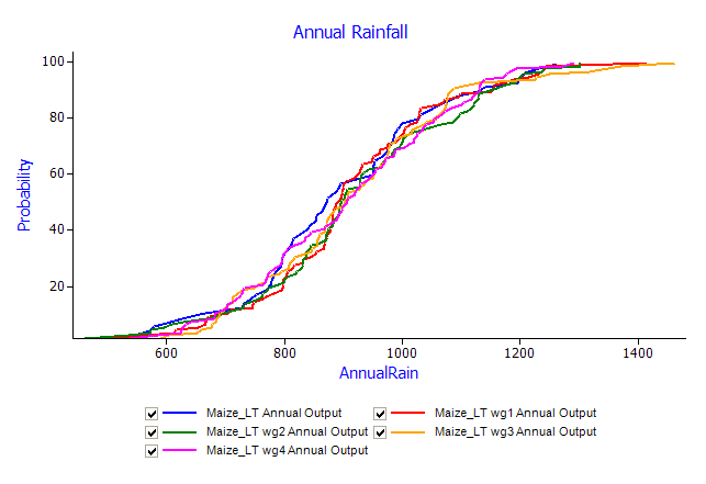
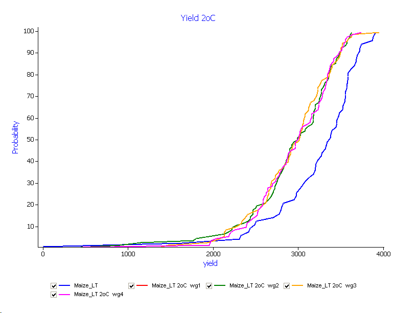
So far, so good – this is what the generator should be able to do. But there’s a different story emerging from a graph of in-crop rainfall. You need to point the ApsimFileReader node at the harvest report files for this:
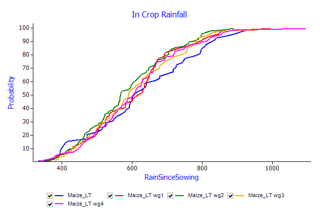
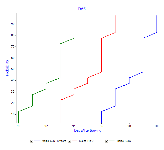
The CDFs are quite different above the median. The key to understanding the difference is in maturity times:
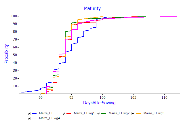
As maturity is governed by temperature (accumulated thermal time), we realise we’ve stumbled across a ‘feature’ of the generator: that while the isolated statistical properties of maximum and minimum temperature are correct, they are not linked (ie temperature range) and as a result the plant model exhibits different behavior.
Stochastic generators and change projections
So far, we’ve examined the generator’s ability to characterise the current climate. The next step is to apply some sort of perturbation to the generator and examine its effect on our cropping system.
In the same area are two sets of change projections (4 replications of each weather sequence):
Chitedze Plus 1: 90% rainfall, +1oC temperature rise
Chitedze Plus 2: 75% rainfall, +2oC temperature rise
The procedure to examine these projections is the same as above – start by creating linked simulations that each use a unique weather sequence.
- Create 4 linked duplicates of the simulation. In each duplicate, unlink the met file component and point to each of the ChitedzePlus1-WG(1,2,3,4).met files in the workshop folder.
- Drag an Empty Manager component from the Management folder in the Standard Toolbox onto the first duplicate. On it’s init tab, set the ambient CO2 level to 450.
- Create links to this node in each of the duplicates.
- Run the simulations
- Create a CDF plot under the top simulations node. In the ApsimFileReader node (Plot -> GDProbability -> “ApsimFile Reader”), select (via the browse button) only the 5 annual output files (xxxx Annual Output.out). In the Plot node, select AnnualRain as the X variable.
- Create another CDF of harvest yields. Select the harvest output files via the browse button in the ApsimFileReader object.