
APSFarm simulations
This exercise uses APSFarm, the whole farm/household configuration of APSIM. In this exercise we will examine whole farm resource allocation questions. A baseline model of a smallholder farm has been constructed, and a number of “what if” scenarios will be explored:
- What is the minimum percentage of sole maize on the farm that provides food security in 90% of years?
- How would this change if fertilisers are used?
- How would that change if CA practises were implemented?
- How would this change assuming a 2050 climate change scenario?
In the workshop folder, you’ll find a simulation file “APSFarm Maize Bean Kakamega.apsim” that has a handful of simulations inside. Of note is that these simulations each have two fields, and at the top level new components have been added: a farm manager, labour, and economics – as distinct from a conventional simulation where managers are in each field.
Unlike the conventional single field rotation, the manager (in the “Crop Management” node) uses a graphical representation of the crop rotation to describe when fields are sown, harvested or are left in fallow (i.e. no crop).
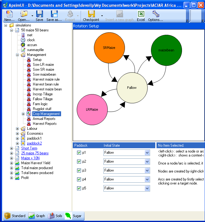
The simulation starts in a “Fallow” state – and tries to change to one of the coloured states as soon as associated rules permit. These rules are shown when one of the arrows between states is clicked.
In the case of “MaizeBean”, the first rule line calls a function (defined in the “Sow maizebean” node), the second line only allows the transition if the paddock under consideration is “paddock1” – so in this simulation, the maize bean intercrop is only considered for paddock 1.
The parameters for sowing (in the “Sow maizebean” node) are similar to before – date windows, planting rainfall, and sowing parameters for each crop.
Of note is that a cost of sowing is defined – the economics component works on the principle that “every management operation has a cost or price associated” – so this cost must be described in detail.
Costs are also associated with labour – when the crop is sown, two labour “operations” are performed – a pre sow tillage, and sowing itself. The work rates are described in the labour component – under the “operator 1” node – where the areal rate and the maximum daily hours are used to calculate a “duration” and “cost” for a given area. Tillage operations incur a labour cost.
Back in the Management “Setup” node we define the areas of each field – i.e. the effective area of each cropping system – by default 0.5ha has been allocated to each enterprise i.e. the sole maize crop, and the maize-bean intercrop.
The aim of this exercise (after verifying that the system is performing in a sensible manner) is to vary these proportions in order to find the food security threshold.
After running the simulation, the CDF of maize harvest yields shows the simulated maize yields and the min/average/max yields expected.
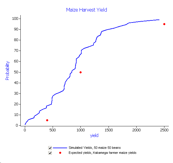
This chart is structured differently from the previous single paddock simulations – it uses a filter component to examine only the yields from paddock 2 – the continuous maize paddock. Removing the filter includes the yields from the first paddock on the CDF.
- Make a copy of the entire Maize Harvest Yield chart to compare later
- Drag a copy of the ApsimFileReader onto the GDProbability reader,
- Delete the Filter component.
Note that charts in these multipaddock configurations do not find data automatically – you have to use the “Browse” buton on the ApsimFileReader component to point at the specific files in question.
Why does including the the yields from paddock 1 (the bean intercrop) raise the CDF?
Of interest is the “50 maize 50 beans cashBook.csv” file produced. You’ll have to open this in Excel. Are economic costs and prices are sensible?
Finally, annual farm production is shown the last 3 charts – total maize and bean tonnages, and profit. In these charts, the first year is discarded (via another filter component) as it only includes the SR season.
Further exercises
- make two linked simulations and change the proportion of intercrop (i.e. maizebean, paddock1) 25/75, and 75/25. Examine the total maize produced and total beans produced CDFs – these are tonnages from the whole farm.
- make another set of linked simulations and apply increasing N (eg 5, 10, 30 Kg NO3) to the maize crops. Is there a contribution from the bean crop?
- Now we want to test what would be the impact of adopting CA practices on the farm, i.e. retaining residues, avoiding tillage, and using RoundUpbefore planting and during the fallow to control weeds.
Make a copy of the short term simulation,
In each of the Management Sowing components, set the “Do xxx tillage operations” to “no”.
Disable the incrop and fallow tillages.
Run the simulation and examine the outputfile component and its charts – it has surface cover and residue weight for both paddocks.
Is there a benefit from the extra stored water?What have you learnt here? What is the additional value of adopting CA practices, and herbicides?
A final exercise will look at estimate what would be the impact of climate change on the original farm (50-50%) under conventional tillage with the use of fertilisers, compared with the CA with the use of fertilisers and herbicides. Follow the procedure outlined in the Climate change projections exercise to drop a “Climate Control” component in the standard toolbox onto the simulation, and make the necessary changes. To add CO2 sensitivity to the bean crop, you’ll have to use a ini file component from the Structural folder in the standard toolbox, and use the fababean-CO2.xml file from the workshop data.