
Fallow Water Balance (SIMLESA)
In this exercise you will explore the major elements of interest in soil water balance during a fallow – soil water storage, drainage, runoff, and evaporation. Changes will be examined over a one year period in the Kakamega district of western Kenya. The examples assume you have read and walked through the Introduction to APSIM UI.
- Create a new simulation using a Continuous Maize Simulation as a starting point.
- Choose Kakamega2010 weather (c:\apsim_workshop\met_files)
- Starting date: 1/9/2002 Ending date: 31/12/2002
- Delete the soil from within the paddock node (“Soil” – a generic Australian Black Earth).
- From International toolbox, find and drag a “Kenya, Masii district Sand, Alfisol (PAWC = 87mm, 1.8m)” soil description onto the ‘paddock’ node of the simulation tree, (located under Soils -> Kenya) removing the existing soil description after the addition. Rename the soil to something short like ‘Sand’. If you like you can also reorder the soil component so it comes straight under the paddock.
- Set the starting water to 50% full – filled from the top. (expand the soil branch to see InitWater – i.e. click the “+” next to Sand)
- At the Initial nitrogen node, set the starting NO3 to 10 kg/ha (i.e. 6 and 4 in the 0-20 and 20-200 layers) and starting NH4 to 5 kg/ha (i.e. 4 and 1 in the two layers).
- Check that the default initial residue type is ‘maize’ and the mass is 0 kg/ha. (at ‘surface organic matter’ node)
- Delete the Fertiliser, Maize and Manager components out of the simulation. They are not needed for a fallow run.
- Select the outputfile’s “My Variables” subcomponent. Choose these variables to report (after removing the old ones):
Component Variable name Clock dd/mm/yyyy as Date Year Day Met Rain Sand ESW – Extractable soil water (mm) ES – Evaporation Runoff DRAIN – Drainage NO3 – summed over profile (Do this by putting () next to the name in the “Variable name” column) eg. no3() (click “?” button next to variable list for more info) DLT_N_MIN – N mineralised – summed over profile Surface organic matter SURFACEOM_WT – Weight of all surface organic materials. SURFACEOM_COVER – Fraction of ground covered by all surface organic materials. - Select the “My Variables Events” subcomponent. Choose “end_day” reporting frequency for the output file. This can be found under the “Clock” component filter.
- Rename the simulation to something more meaningful: Sand Fallow.
- Save the simulation file as Fallow water balance.apsim
- Run the simulation.
- Create a graph of Date vs ESW. To do this, click on the Graph Toolbox at the bottom of the window to open the toolbox. Then drag in an XY component onto the output file in your simulation. Click on the “+” symbol next to XY component to expand the node. Click on the Plot component. In the Plot window click on the X variables square to make sure the background of the square is pink. Now click on the “Date” column heading. It should appear in the list in the square. Now click on the Y variables square to make its background pink. Click on the esw column heading. It will be added to the Y variables square. To have a clean line plotted with no points, under “Point type”, choose “None”. Now click on the XY component to view the graph.
- Once you have created a chart it is possible to make modifications by adding new variables. It is also possible to mix the type of plots used on a graph. As an example, we will add rain as a bar chart on the Y2 axis. To do this, drag “plot” onto the XY node to create a duplicate, ‘plot1’. At ‘plot1’, remove esw and add rain as the y variable. To make the “rain” appear on the right hand axis, click rain in the square to highlight it, then “right” mouse click on it again. In the popup menu click on “Right Hand Axis”. Select “bar” chart from “type” drop_down menu. Select XY node to see the line and bar chart combination.
- Rename the XY graph node to ‘Soil_water_storage’
The graph should show the ESW (in mm) increasing with day of year. The sudden increases are due to rainfall events and the declines to evaporation and drainage loss. The distribution of daily rainfall amounts helps see this more clearly.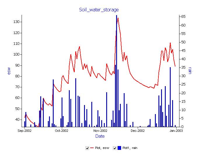
We can also examine other components of the simulated soil water balance.
- Drag ‘Soil_water_storage’ to the outputfile node to make a copy of this graphics node. Rename the copy to ‘Runoff_drainage’
- At the Plot1 node underneath the ‘Runoff_drainage’ graph, remove rain from the Y variables box. Add runoff and drain to the Y variable box. Put both on the right hand axis (right click on the variable) to create a plot similar to the below figure.
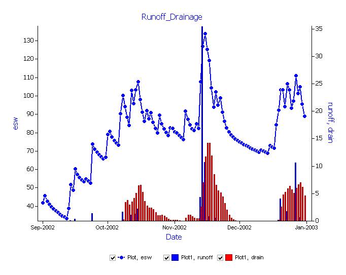
Small amounts of runoff occur early in Sept-Oct, increasing to higher levels in Nov-Dec. Drainage begins sometime after the first runoff, once the soil profile is near full. (Remember, PAWC for this soil is 87mm, so the profile is mostly in a saturated state whenever esw is above this limit).
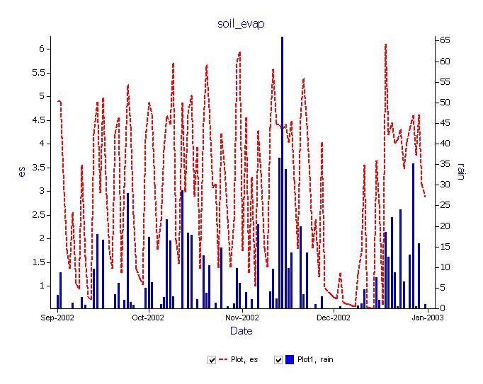
You could also make a plot of soil evaporation. See if you can do this for yourself.
The effect of soil type on the water balance.
Runoff, es and drainage are affected by weather and soil water storage capacity. This run will take an additional soil into account, and compare runoff from both soil types. The user interface still contains all the specifications provided for the previous simulation.
If you drag the Sand Fallow node in the Simulation Tree to the top node Simulations, a copy of it will be made and your file will then have 2 simulations in it. e.g.
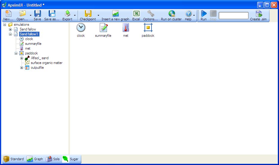
This second simulation can then be modified to add the characteristics of a Clay loam soil.
- From International toolbox, find and drag the “Kenya, Masii district. Clay loam, Alfisol (PAWC = 137mm, 1.8m)” soil onto the paddock in the simulation tree and then remove the old soil. It is important you drag in a new soil BEFORE you delete the old one, otherwise the simulation will lose all your soil reporting variables. Also remember to rename your soil to something shorter – eg Clay
- Since now we have a new soil we will need to go and set the initial soil water (InitWater) to 50% filled from top and initial soil nitrogen (Initial nitrogen) to NO3 to 10 kg/ha and NH4 to 5 kg/ha, as before. When you delete soils you also delete the initial soil water conditions and initial soil nitrogen conditions so these will need to be set similar to the conditions of the “Sand” soil.
- Rename the simulation to Clay Fallow.
- Save the simulations.
- Run APSIM for the Clay soil simulation.
- Graph both the output files by dragging an XY graph onto the top node Simulations in the simulation tree. By placing the XY graph under the Simulations node, all output files in the simulation area will be available for plotting – in this case, the Sand and Clay outputs.
- Create a graph of date vs esw and runoff(cumulative, right hand axis). To make the runoff cumulative, it is the same procedure as to make the rain appear on the right hand axis. Only select “Cumulative” from the popup menu instead of “Right Hand Axis”. Set “Point Type” to “None”.
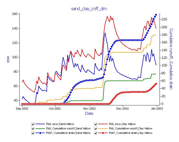
The above figure includes a plot of drainage for the 2 soils. See if you can also add ‘drain’ as shown above to your esw-runoff plot. (Hint: create a plot1, do cumulative and right hand axis and choose ‘circles’ under Point Type)
The clay soil has higher runoff than the sandy soil for all simulated events. Cumulative runoff for the sand is approx 80mm. For the clay it is 180mm. Is this what you might expect, given the same rainfall and 50% full profiles as starting conditions?
To begin, the clay soil has higher ESW because of its higher water holding capacity and the fact that both soils were initialised at 50% of capacity. By Oct the esw in the sand is the same as in the clay, meaning it has captured more of the rainfall. How could this happen?
The sandy soil attains field capacity (87mm) by mid-Oct and drainage from the bottom soil layer begins around this time. In the absence of a growing crop, the seasonal drainage is over 220mm. The clay soil attains field capacity (134mm) almost 1 month after the sand, and retains a higher esw than the sand for the remainder of the season. This is due to a combination of higher PAWC and less drainage beyond the root zone compared to the sand (cumulative clay soil drainage is less than 60mm.)
Additional investigation: explore what effect curve number has on the water balance. eg. for the sandy soil, change curve number from 73 to 85 in the Soilwat node.