SWIM3

SWIM3: Model Documentation

N. I. Huth, K. L. Bristow, K. Verburg

Information taken from Huth, N.I., Bristow, K.L., Verburg, K., 2012. SWIM3: Model use, calibration, and validation. Transactions of the ASABE 55, 1303-1313.

Introduction

SWIM3 is the latest release in the family of SWIM (Soil Water Infiltration and Movement) models developed for simulating water and solute movement within soils.  These models have been used predominantly for studies into management options for water and solutes in agricultural systems or for evaluating alternate numerical methods for efficiently solving complex systems of flow equations.  SWIMv1 (Ross, 1990b) provided an efficient solution to the 1-dimensional Richards’ equation for the simulation of water movement and uptake by plants.  SWIMv2 (Verburg et al., 1996b) extended the functionality of SWIMv1 through the provision of a wider range in boundary conditions, the ability to specify soil hydraulic properties as the sum of simple functions (Ross and Smettem, 1993) described using piecewise cubic approximations (Ross, 1992), and a solution of the convection-dispersion equation for solute transport.  The utility of this model code was further enhanced by its incorporation into the APSIM (Agricultural Production Systems Simulator) framework (Keating et al., 2003) to create the APSIM-SWIM version of the model (McCown et al., 1995; Huth et al., 1996). With this move, SWIM ceased to be developed as a standalone product, but was redeveloped for use as a component within integrated modeling frameworks.  Whilst much of the numerical approach used within the APSWIM-SWIM model was retained from the parent SWIMv2 model, further enhancements were included to facilitate application to various farming systems.  These included the simulation of multiple non-interacting solutes(Verburg et al., 1996a), the effects of surface residues on evaporation or surface sealing (Connolly et al., 2002) and equations for simulating subsurface drains (Malone et al., 2007; Snow et al., 2007) or local groundwater interactions (Paydar et al., 2005b).  SWIM3 builds upon the work of APSIM-SWIM and provides a new approach to specify soil hydraulic properties for a broad range of soil types from simple measures of soil water behavior.  The simplicity of this new approach makes this mechanistically-based numerical model more accessible to farming systems researchers within the APSIM modeling community who, until now, have limited their use of APSIM-SWIM due to perceived difficulties of parameterization.  SWIM3 is developed and maintained within the APSIM Community Source Framework (www.apsim.info) by the APSIM Initiative.  This initiative provides a transparent and open-source approach to combine broadly based collaborative science with best practice software development and maintenance, and science quality control.  APSIM is freely available for research and development, extension or educational use.  APSIM training is provided via regular international workshops as a fee for service activity.  However, all workshop materials, user documentation and a model user support forum are also freely available via the APSIM website (www.apsim.info).

SWIM3 Description

The APSIM modeling framework has been developed to simulate biophysical process in farming systems, in particular where there is interest in the economic and environmental outcomes of management practice in the face of climatic risk, climate change or changes in policy.  APSIM’s component-based design allows individual models to interact via a common communications protocol (Moore et al., 2007).  The role of SWIM3 within an APSIM simulation is to calculate fluxes and storage of soil water and solutes and to communicate this information to other models within the simulation. Whilst SWIM generally uses much smaller time steps in computing its numerical solutions, most communications to other models within a simulation occur on a daily frequency.    SWIM3 is available for use in APSIM Version 7.3 or later.

SWIM3 is a 1-dimensional lumped physically-based model.  Some sub models within SWIM3 capture simple spatial processes and so it can also be described as a quasi 2-dimensional model.   SWIM3 provides a 1-dimensional simulation of water fluxes through a numerical solution to Richards’ equation (Richards, 1931) (Eq. 1)

(1)

 

where θ is volumetric water content (cm³cm^-3), x and t describe space (cm) and time (h), K is hydraulic conductivity (cm h^-1), z and ψ are the gravitational and matric potentials (cm), and S is the source/sink term for water  (cm³cm^-3h^-1).  Solute fluxes are calculated using a solution to the Convection-Dispersion equation (Eq. 2)

(2)

 

where c and s are solute concentrations (ppm) in solution or adsorbed to the soil surface, D is the combined dispersion and diffusion coefficient (cm² h^-1), q is the water flux (cm h^-1) and ρ is the soil bulk density (g cm^-3), and φ is the source/sink term for solute (ppm h^-1).  The mixed ψ and θ form of Richards’ equation shown in equation 1 is highly non-linear, especially in dry soils, and so it is solved using a hyperbolic sine transform of ψ (Ross, 1990a).  A detailed description of the numerical methods used in solving equations 1 and 2 is included in (Verburg et al., 1996b).

Various losses from the overall water balance, such as canopy interception or losses from irrigation infrastructure are calculated in other modules within APSIM.  Potential crop water use is calculated by each crop model using methods appropriate to the crop being simulated as specified by each crop model developer.  Evaporation, drainage and runoff losses are calculated via sub-models within SWIM3 and incorporated into the numerical solution through the sink term, S.  Evaporation is calculated using the approach of  Campbell (1985) assuming isothermal vapor transport.  Potential evaporation rate is calculated using the method of Priestly and Taylor (1972).  Plant water uptake is calculated using the approach of  Campbell (1985) which treats the soil-plant-atmosphere continuum as a resistance network.  Uptake from each layer is calculated using the analogue of a single cylindrical root surrounded by a homogeneous cylinder of soil (Cowan, 1965). Partitioning of water uptake between layers is obtained by calculation of a xylem potential, up to a species-specific maximum value, required to meet daily plant water demand.  Loss via subsurface drainage networks is calculated using the steady-state Hooghoudt equation (Malone et al., 2007), formulated in a way similar to that found in DRAINMOD (Skaggs, 1989).  Vertical losses from the soil profile are calculated depending on the chosen bottom boundary condition.  A zero matric potential gradient is assumed to exist below the bottom boundary for simulations where no water table exists within the soil profile.  Otherwise, ground water flow is calculated from the simulated water potential at the bottom boundary using a lumped parameter describing the rate of flow per unit potential difference to capture ground water behavior (Paydar et al., 2005b).

Runoff losses were previously calculated in SWIMv1 and SWIMv2 using detailed models of surface water storage and soil surface crust dynamics in response to detailed data on storm rainfall intensity (Connolly et al., 2002).  These approaches often required parameters and input data not available to many users.  SWIM3 makes use of the SCS Runoff Curve Number technique (Hawkins, 1996) for calculating daily runoff losses from more readily available daily rainfall totals.

The convection-dispersion equation (Eq.2) is used to calculate the fluxes of all solutes within the APSIM simulation (usually NO₃, NH₄, Cl, and Urea).  No interaction or competition for exchange surfaces by solutes is considered.  Adsorption of solute to soil surfaces is specified via a Freundlich isotherm and soil pore space tortuosity effects on solute diffusion are captured in a simple user-defined function of soil water content which can reproduce many of the common forms (Moldrup et al., 2005).

Simulations can be applied to a field, or to a section within a field, depending on the intended use of the model.  Field variability is captured within the lumped parameterization approach.  If field variability is large, separate simulations are conducted for the main soil types within the field and results are aggregated in an appropriate manner.  The timescale of an APSIM simulation generally ranges from a few days to over a century in duration if suitable input data, such as weather information, exists.  The user selects the depth of the soil profile to be simulated and the way in which this profile is discretized into soil layers for numerical solution.  Soil properties can be input at different levels of spatial information (detailed spatial disaggregation vs simple soil horizons) and these are mapped into the simulation layer structure by the user interface, ensuring conservation of mass of water and solutes, and appropriate interpolation of model parameters.

SWIM3 Calibration and Validation

SWIM3 Calibration

SWIM3 has been developed for use within the APSIM modeling framework and so the requirements for model parameterisation are set by the requirements for farming systems analysis.  Soil water balance is a critical component in the simulation of many farming systems and the functional requirements of soil water models vary.  Because of this, APSIM has provided both detailed (e.g. Richards’ equation) and simple (e.g. capacity or ‘bucket’) models to suit the various problem domains and uses of the model.  Detailed models rely on information on soil hydraulic properties, which are often determined using laboratory techniques, pedotransfer functions or inverse methods.   From these basic properties the hydraulic behavior is determined via solutions to the flow equations.  However, history has shown that simple soil water models are more extensively used, despite their shortcomings, because they are easier to parameterize and provide a much simpler conceptual model of soil water behavior.

Simple ‘cascading’ water balance models, such as the Soilwat model (Probert et al., 1998), make use of well known properties of soils such as the Drained Upper Limit (DUL) or Field Capacity, the Lower Limit (LL) of plant water extraction, and the saturated water content (SAT) and saturated hydraulic conductivity (K_S).  The difference between DUL and LL is referred to as the Plant Available Water (PAW) content and is a very important soil property in agronomic assessment.  The first advantage of this way of describing soils is that these parameters align very closely to the conceptual model employed by many users of farming systems models (Gardner, 1988; Dalgliesh and Foale, 1998).  The second advantage is that long standing and geographically broad usage of these simple models provides a very large database of readily accessible soil data for use with these simple models.  Furthermore, options exist for deriving properties from simple in situ field measurements (Dalgliesh and Foale, 1998) and so many modelers are continually adding to the information available for future model users.  However, the simulation of some problem domains requires more detailed hydrological models to describe certain boundary conditions (e.g. fluctuating water tables), detailed solute fluxes (e.g. salt or nitrate leaching), complex flow processes (e.g. sub-surface drains), or processes occurring at much smaller time and spatial scales.  There is therefore an advantage to be gained from providing a means for farming systems modelers to use a Richards’ equation model within their agronomic understanding of soil function.  SWIM3 provides such an approach.

The values of SAT, DUL and LL are used to describe three points on the soil water retention curve, θ(ψ). These three water contents are assumed to correspond to soil matric potentials of 1 cm, 100 cm and 15000 cm respectively, though the user can choose to vary the value used at DUL.  A fourth and very important point on the retention curve is the zero water content assumed in oven drying of soil samples for determination of soil water content.  The nature of the retention curve approaching dryness is important for simulating evaporation from the soil surface (Ross et al., 1991).  The corresponding matric potential for oven dry soil, assuming air of 25° C and 50% relative humidity, is 6.09×10⁶ cm, though the impact of these assumptions is likely to be low (Ross et al., 1991).  Two further assumptions are made from general observations of soil water retention data. The slope of the retention curve is assumed to be zero at saturation and almost constant between LL and oven dry.  From these six pieces of information a series of monotonic cubic Hermite splines are constructed for describing the retention curve across the entire water range (See Appendix for more details).  The use of splines ensures that the retention curve exactly matches the model user’s specification of ranges of water contents for near saturation, plant available and near dry conditions.

 

The hydraulic conductivity function, K(θ), is inferred from the model user’s specification of DUL and K_S.  K_S describes the drainage rate at saturation.  By definition, DUL describes the water content at which drainage rate is reduced to some nominal low value, hereafter K_DUL.  This information then provides two points on the soil hydraulic conductivity function with which we develop a two-region model of hydraulic conductivity incorporating the effect of macropores and micropores.  This approach is very similar to the three-region model of Poulsen et al.(2002).  Both this model, and that of Poulsen et al. (2002), avoid errors caused by extrapolating a single function from saturation to dry soil by anchoring and interpolating the function at intermediate water contents using extra information.  Here, we assume that the conductivity function is related to the retention curve when the soil water content is below DUL and that the conductivity is a notional value of 0.1 mm d^-1 at DUL. A function for macropore contribution to K is calculated such that it is significant only above DUL, and results in total conductivity equaling K_S at saturation.  This approach ensures that drainage rates approach K_S at saturation and that water content approaches DUL after drainage (Gardner, 1988). A more detailed description of the method is included in the Appendix.

Figure 1 illustrates how the four moisture contents (SAT, DUL, LL, Oven Dry) are used to create a continuous soil water retention curve (Fig. 1a) and how the two-region conductivity function is constructed from the SAT-K_S and DUL-K_DUL pairs (Fig. 1b) representative of a silt-loam soil.

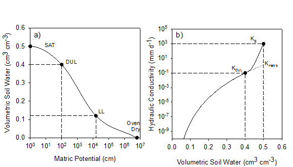
Figure 1. Demonstration of how basic soil properties (SAT = 0.5 cm³cm^-3, DUL= 0.4 cm³cm^-3, LL= 0.12 cm³cm^-3, Oven Dry, K_S=1000 mm d^-1, K_DUL=0.1 mm d^-1) are mapped into continuous hydraulic property functions for a) water content and b) hydraulic conductivity. See appendix for definition of K_matrix.

Calibration Parameters

The main parameters used in calibrating SWIM3 are therefore SAT, DUL, LL and Ks.  Several methods are commonly used to determine these parameters.  SAT is often estimated as a fixed proportion of the total porosity of the soil calculated from the soil bulk density.  Bulk density is a mandatory parameter for several APSIM models and so it is not a data requirement particular to SWIM3.  DUL and LL are often determined in the field: DUL via measurement of soil water content after an extended period of drainage following saturation and LL after maximal drawdown of soil water content by plants (Dalgliesh and Foale, 1998). Alternatively DUL and LL can be estimated from laboratory measurements of soil water content at 100 cm and 15000 cm matric suctions respectively (Gardner, 1988). Finally, SAT, DUL and LL can all be estimated from regular observations of soil water content including periods of wetting up and drainage, and periods of drying down by plants.  Soil water content will often vary between SAT and DUL during periods of frequent rewetting, and decrease to LL during periods of high crop water use and minimal water input.  In cases where long term information on soil water variation is available, rapid estimates of soil hydraulic properties can be obtained from direct interpretation of soil behavior.  This approach will be demonstrated in the two case studies below.

The saturated conductivity of the soil, K_S, can be estimated from infiltration studies, laboratory measurements or relationships based on soil texture.  As stated above, the method used to derive the conductivity function within SWIM3 removes some of the sensitivity of the model to errors in estimates of K_S by anchoring the conductivity curve at DUL.  The model will still be sensitive to estimated K_S values near saturation and so the parameter will be important under situations of high water input.  Under dry land conditions, parameters for soil water holding capacity are likely to be more important.

The following remaining parameters are of some importance.  The runoff curve number (Hawkins, 1996), used in partitioning rainfall between infiltration and runoff, is usually derived from guidelines based on soil texture and soil surface characteristics (Ringrose-Voase et al., 2003).  Many of the parameters for the convection-dispersion equation are taken from the literature or physical tables and so are available as default values for the user.  Defaults are also provided for parameters used in the numerical solution of Richards’ equation.  These include error tolerances, limits for the magnitude in iterative increments, space weighting factors and user selections for handling numerical dispersion and oscillations.  In most cases the recommended default values can be adopted by the model users.

It should be noted that a great number of other parameters are required by other models within an APSIM simulation.  These are outside the scope of this paper.  However, the reader can refer to other publications for information on parameters for crop growth (Robertson et al., 2002; Wang et al., 2002),  soil organic matter and nutrient dynamics (Probert et al., 1998; Huth et al., 2010), rules for agronomic management (Keating et al., 2003) and various climatic data (Jeffrey et al., 2001).

 

Discussion

The strength in SWIM3 comes from the mechanistic numerical model based on solutions of the 1-dimensional Richards’ and Convection-Dispersion equations.  The main advantages of SWIM3 over the early versions of the model come from its implementation within the APSIM framework.  The large number of crop and soil modules available to the user allows the SWIM water balance to be used in model applications across a wide range of problem domains.  These benefits have been used in many previous studies using the earlier APSIM-SWIM model as mentioned in the introduction to this paper.  However, this new implementation of the SWIM model brings with it new benefits arising from the approach used for soil parameterization.  SWIM3 can now be parameterized using fairly simple measures of soil attributes for which formalized techniques are readily available (Dalgliesh and Foale, 1998).  These attributes, which describe the plant available water holding capacity of a soil, are also very important determinants of the productivity of a soil, especially for dry land farming systems (Dalgliesh and Foale, 1998).  It is therefore logical that these parameters will also be very important determinants of modeled crop production.  Previous studies have shown that grain yield changes in response to water supply by an average 20 kg ha^-1 mm ^-1 for wheat in southern Australia (French and Schultz, 1984).  Responses from crop models are likely to be comparable and so errors in predictions of soil water supply will likely cause significant errors in crop production.  However, parameterization of SWIM3 directly from data on plant available water contents provides the user with close control of modeled water balance and the resulting crop production.

As has been shown in this paper, the model can also be very easily parameterized from very simple data on soil water behavior such as observed ranges in soil water content.  These approaches have been used with simple ‘cascading’ water balance models such as SoilWat (Probert et al., 1998) in APSIM.  In this case, we use this same approach of parameterization from simple observations of soil water behavior but combine this with a more robust physically-based numerical model.  One consequence of this approach is a reduced number of soil parameters to that required by the cascading water balance for some soil processes.  For example, two parameters used in Soilwat to describe evaporation, two for unsaturated flow, and one for near-saturated water flow are not required when we parameterize SWIM3 from the same basic field observations because these processes are now captured by the solution of Richards’ equation.

 

One weakness of SWIM3 when compared to the simpler soil water balance models is the increased execution time required for the iterative solution of a series of highly non-linear differential equations.  In many applications this computation overhead is of little consequence and the benefit of the extra model capabilities outweighs this cost.  However, this will be a limitation to its use for large scale spatial analyses or large suites of long term simulations, as is increasingly required of modern farming systems models.  Solutions to this constraint are available (Ross, 2011) and will be explored for a future release of the model.  A second weakness of the model is the lack of any consideration of the impact of soil chemistry on soil hydraulic properties.  Chemical impacts on hydraulic properties, as is the case in sodic subsoils, are captured using empirical relationships in simple water balance models (Hochman et al., 2007).  The effects of soil chemistry on the assumptions used in describing soil hydraulic properties in SWIM3 will be considered in future work.

This paper also highlights the issues in model parameterization.  While there is much value in efforts to provide laboratory measurement or numerical optimization of soil hydraulic properties, we have demonstrated that simple logic applied to soil water behavior can be used in a similar way.  Soil properties can be deduced from soil behavior.  Both approaches, measurement or rational deduction, are valid (Williams et al., 1991).  A soil’s water content after drainage, and its plant available water holding capacity, are often consistent and well understood emergent properties of a soil and so model parameterization should take these into account in a simple but meaningful way.  The method employed in this model, and the case studies shown above, provides such a framework.

Future Developments

Future development of SWIM3 will address the deficiencies identified above to provide increased numerical efficiency and the effect of soil chemistry on soil hydraulic processes.  There are also efforts underway to allow rapid laboratory or field measurements to further inform model parameterization using commercially available apparatus.  Modelers interested in assisting further development of SWIM3 can do so via contacting the authors or involvement in the APSIM Community Source Framework (www.apsim.info).

Acknowledgements

Peter Ross provided much of the specialist design of the numerical methods used in SWIMv2 and hence SWIM3.

References

 

Campbell, G.S. 1985. Soil Physics with BASIC. New York, USA: Elsevier.

Connolly, R.D., M. Bell, N. Huth, D.M. Freebairn, and G. Thomas. 2002. Simulating infiltration and the water balance in cropping systems with APSIM-SWIM. Australian Journal of Soil Research 40:221-242.

Cowan, I.R. 1965. Transport of water in the soil-plant-atmosphere system. Journal of Applied Ecology 2:221-239.

Dalgliesh, N.P. and M.A. Foale. 1998. Soil Matters – monitoring soil water and nitrogen in dryland farming. Toowoomba, Australia: Agricultural Production Systems Research Unit.

Fritsch, F.N., Carlson, R.E. 1980. Monotone piecewise cubic interpolation.  Siam Journal on Numerical Analysis 17: 238-246.

Gardner, E.A. 1988. Soil Water. In Understanding soils and soils data, 153-186. I.F. Fergus ed., Brisbane, Queensland : Australian Society of Soil Science Inc.

Hawkins, R.H. 1996. Runoff Curve Number: Has It Reached Maturity? Journal of hydrologic engineering 1:11-19.

Hochman, Z., Y.P. Dang, G.D. Schwenke, N.P. Dalgliesh, R. Routley, M. McDonald, I.G. Daniells, W. Manning and  P.L. Poulton. 2007. Simulating the effects of saline and sodic subsoils on wheat crops growing on Vertosols. Australian Journal of Agricultural Research 58: 802-810.

Huth, N.I., B.A. Keating, K.L. Bristow, K. Verburg, and P.J. Ross. 1996. SWIMv2 in APSIM: An integrated plant, soil water and solute modelling framework. Proc. 8th Aust. Agron. Conf., p. 667. Toowoomba, Australia: Australian Agronomy Society.

Keating, B.A., P.S. Carberry, G.L. Hammer, M.E. Probert, M.J. Robertson, D. Holzworth, N.I. Huth, J.N.G. Hargreaves, H. Meinke, Z. Hochman, G. McLean, K. Verburg, V. Snow, J.P. Dimes, M. Silburn, E. Wang,  S. Brown, K.L. Bristow, S. Asseng, S. Chapman, R.L. McCown, D.M. Freebairn and  C.J.Smith.  2003. An overview of APSIM, a model designed for farming systems simulation. European Journal of Agronomy 18: 267-288.

Malone, R.W., N. Huth, P.S. Carberry, L. Ma, T.C. Kaspar, D.L. Karlen, T. Meade, R.S. Kanwar, and P. Heilman. 2007. Evaluating and predicting agricultural management effects under tile drainage using modified APSIM. Geoderma 140: 310-322.

Moldrup, P., T. Olesen, S. Yoshikawa, T. Komatsu, A.M. McDonald and D.E. Rolston.  2005. Predictive-descriptive models for gas and solute diffusion coefficients in variably saturated porous media coupled to pore-size distribution: III. Inactive pore space interpretations of gas diffusivity. Soil Science 170: 867-880.

Moore, A.D., D.P. Holzworth, N.I. Herrmann, N.I. Huth and M.J. Robertson. 2007. The Common Modelling Protocol: A hierarchical framework for simulation of agricultural and environmental systems. Agricultural Systems 95: 37-48.

Mualem, Y. 1976. New model for predicting hydraulic conductivity of unsaturated porous media. Water Resources Research 12: 513-522.

Paydar, Z., N. Huth, and V. Snow. 2005b. Modelling irrigated Eucalyptus for salinity control on shallow watertables. Australian Journal of Soil Research 43:587-597.

Poulsen, T.G., P. Moldrup, B.V.  Iversen, and O.H. Jacobsen. 2002. Three-region Campbell model for unsaturated hydraulic conductivity in undisturbed soils. Soil Science Society of America Journal 66:744-752.

Priestley, C.H.B. and R. J. Taylor, 1972. On the assessment of surface heat flux and evaporation using large scale parameters. Monthly Weather Review 100: 81-92.

Probert, M.E., J.P. Dimes, B.A. Keating, R.C. Dalal and W.M. Strong. 1998. APSIM’s water and nitrogen modules and simulation of the dynamics of water and nitrogen in fallow systems. Agricultural Systems 56:1-18.

Richards, L.A. 1931. Capillary conduction of liquids through porous mediums. Physics-a Journal of General and Applied Physics 1: 318-333.

Ross, P.J. 1990a. Efficient numerical methods for infiltration using Richards equation. Water Resources Research 26:279-290.

Ross, P.J. 1990b. SWIM – A simulation model for soil water infiltration and movement. Reference manual to SWIMv1. Canberra, Australia: CSIRO Division of Soils.

Ross, P.J. 1992. Cubic approximation of hydraulic properties for simulations of unsaturated flow. Water Resources Research 28:2617-2620.

Ross, P.J. 2011. Numerical Solution of the Continuity Equation for Soil Water Flow Using Precomputed Steady-State Fluxes. Vadose Zone Journal 10:760-766.

Ross, P.J. and K.R.J. Smettem. 1993. Describing soil hydraulic properties with sums of simple functions. Soil Science Society of America Journal 57:26-29.

Ross, P.J., J. Williams and K.L. Bristow. 1991. Equation for extending water-retension curves to dryness. Soil Science Society of America Journal 55: 923-927.

Skaggs, R. 1989. DRAINMOD user’s manual. Interim Technical Release. Raleigh, NC: Biological and Agricultural Engineering Department, North Carolina State University.

Snow, V.O., D.J. Houlbrooke and N.I. Huth. 2007. Predicting soil water, tile drainage, and runoff in a mole-tile drained soil. New Zealand Journal of Agricultural Research 50:13-24.

Verburg, K., P.J. Ross and K.L. Bristow 1996b. SWIM V2.1 User Manual: Divisional Report No. 130. Canberra, Australia: CSIRO Division of Soils.

 

Appendix

Describing The Soil Water Retention Curve using Hermite Splines

SWIM3 uses a series of monotonic cubic Hermite splines (Fritsch and Carlson, 1980) to describe the soil water retention curve.  Values for θ are interpolated between the four points for 1) Saturation, 2) Drained Upper Limit, 3) Lower Limit, and 4) Oven Dry.  The method is as follows:

i) Calculate the slope of the secant lines between each successive point

ii) Calculate the slope at each successive point as the average of the secants either side of this point.

 

iii)                  The resultant cubic spline will not be monotonic if either of the following is true

If so set

Where

iv) Interpolate the value of θ following the standard method for evaluating a cubic Hermite spline for the relevant region between ψ_i and ψ_i+1 within the interpolation set.

Where

and the basis functions for the cubic Hermite spline are:

 

Describing Hydraulic Conductivity from Basic Drainage Information

SWIM3 describes hydraulic conductivity as the sum of two functions describing the conductivity of the soil matrix and macropores (Ross and Smettem, 1993).  The function for the soil matrix is related to the shape of the soil water retention curve (Mualem, 1976) as expressed by Campbell (1985).  A simple power function is used for the contribution of macropores.

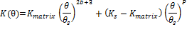
where

The contribution of the micropore component is calculated from the assumption that the conductivity at DUL (K_DUL) is almost entirely due to the soil matrix.  Thus, the conductivity of the soil matrix component at saturation is

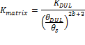
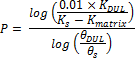
The value of P is calculated using the assumption that, at the drained upper limit, the conductivity of the macropores is negligible.  A value of P is therefore determined such that the conductivity of the macropores at DUL contributes only 1% of the overall value of K_DUL.