
SurfaceOM
The processes included in the SurfaceOM module are depicted in Figure 1.
Briefly, the above ground material can be burnt (or removed from the system in some other way, e.g. baling), incorporated into the soil during tillage operations, or decomposed.
Above ground residues are considered as consisting of a mixture of one or more different materials (or component parts), each of which is defined in terms of:
- Mass (kg/ha)
- Overall C:N ratio ()
- Overall C:P ratio ()
- Standing Fraction (0-1)
- Type (eg wheat, lucerne, eucalyptus leaves etc) – from which SURFACEOM will determine the following information:
- Overall Carbon fraction (0-1)
- Specific Area (ha/kg)
- Potential Decomposition Rate (/day)
- Mineral Composition (nh4, no3,and po4 (in ppm))
- C,N,P fractions in each of the fresh organic matter (FOM) pools (i.e. carbohydrate, cellulose, lignin)
SURFACEOM module outputs can either refer to the entire mixture of surface materials, or to specific components.
When new material is added (e.g. at harvest), the material will either enter an existing surface organic matter component (eg wheat) or may start a new component, if that residue is a new addition to what is already present in the system (for example, wheat trash being added to existing lucerne residues, at harvest).
Each component is kept separate for calculations of C:N ratio, decomposition, and specific area.
An overall effective cover value (0-1) is calculated using all surface organic matter components present, for the purposes of subsequently calculating surface material effect on soil evaporation and runoff.
If a particular surface organic matter type has soluble inorganic N components (NO3-N and NH4-N), these may be transferred to the respective soil pools by leaching due to rainfall or irrigation.
The cumulative amount of rain and irrigation to transfer all of the soluble components is specified as an input; the amount leached is proportional to cumulative rain.
It is possible to specify that a certain proportion of any particular surface organic matter is ‘standing’, that is, inert from the processes of decomposition.
The default value for this proportion is zero, in other words, all the material is decomposable.
See section below on ‘Standing/Lying Components’
Tillage results in a transfer of some surface OM into the soil FOM pool.
With tillage, surfaceOM N and C is incorporated into soil layers to the nominated tillage depth, and added to the respective soil mineral N and the fresh organic matter pools (FOM).
Incorporated surfaceOM C and N is partitioned into the rapid, medium and slowly decomposing FOM pools according to nominated fractions.
This fractionation is dependant upon the type of OM and so differences between crop residues and animal manures, for example, can be specified.
Decomposition results in loss of some carbon as CO2 and transfer of carbon and nitrogen to the soil.
Decomposition of residues with a high C:N ratio creates an immobilisation demand, which is satisfied from mineral-N in the uppermost soil layers;
in extreme situations, inadequate mineral-N in soil restricts decomposition of residues.

Figure 1. Schematic representation of the processes in the SURFACEOM module. (Note that default values of zero are used for mineral N and P components in plant residues)
Surface Organic Material Decomposition
Decomposition of surface OM’s is calculated using a simple exponential decay algorithm
where the fraction of each component decaying on any day (Fdecomp) is calculated as follows:
Fdecomp = Potential Decomposition Rate x Moisture Factor x Temperature Factor x C:N ratio Factor x Contact Factor
From this fraction, potential amounts of carbon and nitrogen to move into the soil are calculated for each component.
Any module responsible for soil organic matter pools (such as the SOILN module) can use this potential supply of carbon and nitrogen in its calculations.
The actual value of decomposition (that is a final soil limited value) for each component is passed back to the SURFACEOM module and above-ground component pools are updated using this value of decomposition.
The moisture factor for decomposition
The moisture factor affecting decomposition in the SURFACEOM module uses cumulative potential soil evaporation (EOS) to capture the effect that dry residues decompose more slowly than wet residues.
It is assumes that residues dry out at a rate proportional to Eos, and that a critical cumulative evaporation (cum_eos_max) results in residues becoming so dry that decomposition ceases.
Moisture Factor = 1.0 – SEOS/cum_eos_max
The factor is constrained to values between 0 and 1.
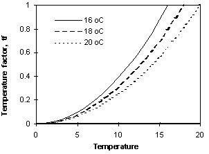
The temperature factor for decomposition
The effect of temperature on residue decomposition is described by:
Temperature Factor = (average air temperature / opt_temp)2
where: average air temperature = (maxt + mint) / 2
This factor is then constrained to values between 0 and 1.
The resultant relationship is shown in the following figure for three values of optimum temperature.
(tf = 20 is the default).
If average temperature is less than zero, the temperature factor is zero.
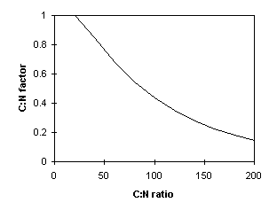
The C:N ratio factor for decomposition
![]()
where
- CN = C:N ratio of surface residues
- CNopt = Optimum C:N ratio for decomposition
- k = coefficient determining slope of curve.
This factor is calculated for individual residue types rather than for the entire mixture and is constrained to values between 0 and 1.
The standard values used with SURFACEOM are k = 0.277 and CNopt = 25.
The resultant curve is as follows:
The soil contact factor on decomposition
Where large amounts of surface residues are present, overall rates of decomposition will be lower.
It is presumed that the material in immediate contact with the soil decomposes more rapidly than that piled on top (a “haystack” effect).
To account for this a Contact Factor discounts decomposition according to the amount of residue.
The relation currently used is based on work by Thorburn et al.(2001) , and involves the concept of a critical mass of surface organic matter at which the “haystack effect” is deemed to become relevant.
It may be summarized as:
- If surfaceom_wt < critical mass then cf = 1.0
or - If surfaceom_wt > critical mass then cf = critical mass/surfaceom_wt
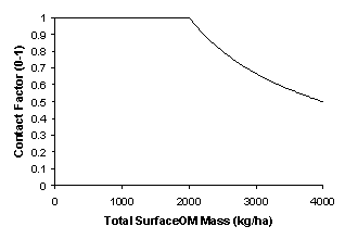
Not all surface residues contribute to this “haystack effect”.
Standing residues are excluded, and some residues on the soil surface can be specified to only contribute partially to the effect.
For example, course woody debris would not contribute but fine leaf litter would.
Tillage of above-ground residues
Residues are incorporated into the soil profile using a tillage command.
For example, the following manager command will incorporate 50% of residues into the top 100mm of soil.
(Note: the following information needs to be specified on a single line in APSIM manager logic)
surfaceom tillage type = ”user_defined”, f_incorp = 0.5 (0-1), tillage_depth = 100. (mm)
Alternatively, the user can specify tillage operations in terms of an implement, with the corresponding values of f_incorp and tillage_depth being defined in the SURFACEOM module’s constants file.
Some examples are:
surfaceom tillage type = disc ()
or
surfaceom tillage type = burn ()
In the “burn” example, the tillage type is specified to incorporate to a zero depth, and the fraction of organic matter specified to be incorporated will be lost from the system.
Each time a “tillage” is specified, all surface organic materials are effected.
If the user is wanting to simulate a situation where only one of the surface materials is incorporated (eg. Digging manure into row spaces between existing crop stubbles) leaving the remainder intact, there is a specific command available called “tillage_single”.
The syntax is as follows:
surfaceom tillage_single name = manure , type = ”disc”()
The “name”refers to the specific name in the system of the surfaceom to be tilled.
Subsequent arguments are as for the standard “tillage” command (see above).
SurfaceOM Cover
SurfaceOM cover is calculated by combining the individual masses of surface OM types and their specific areas (i.e. an area of cover per unit mass)
Currently, both “standing” and “lying” fractions are considered to contribute to cover.
However, increasing amounts of surface OM have diminishing effects due to the additional residue overlaying other residues rather than covering bare soil.
This can be described as:
dC/dS = 1 – C (1)
where
C is the effective fractional residue cover, and
S is the total surface area of residues per unit area
and hence
C = 1 – eS (2)
SurfaceOM Input Parameters
| Name | Units | Description |
| name | – | Individual residue name |
| type | – | Specific residue type (referenced to .ini file) |
| mass | kg/ha | Initial amount of surface OM |
| cnr | – | Initial C:N ratio of surface OM |
| cpr (optional)* | – | Initial C:P ratio of surface OM |
| standing_fraction (optional)* | (0-1) | Standing or inert component of surface material |
* – if optional parameters are not supplied then defaults from constants file are used.
All SurfaceOM module input parameters are arrays, hence several surface OM types can be initially specified as existing in the simulation.
For example:
[all.surfaceom.parameters]
name = wheat_old wheat_new lucerne ! name of surface OM material
type = wheat wheat lucerne ! type of surface OM material
mass = 350.0 2000.0 400.0 ! mass of surface OM (kg/ha)
cnr = 100.0 75.0 35.0 () ! C:N ratio of surface OM
If desired, only a single surface OM may be specified (in similar fashion to the old APSIM RESIDUE2 module), or up to a maximum of 100 materials.
The “name” of the surfaceom is a unique identifier of that surfaceom pool.
The “type” is the specific type of material, used to reference further information for that type.
In other words, there can be several surfaceom’s of the same “type” in the system, but only one instance of each “name” is allowed.
See the above example, where residues from an old wheat crop are present together with new residues from a more recent wheat crop.
They are both of the same “type”, but are considered as separate pools, each with an individual “name”, wheat_old and wheat_new.
When a crop discards leaves/stems etc, they are added to the SURFACEOM module in a pool with the “name” and “type” equal to the crop name, i.e. wheat, chickpea.
SurfaceOM Standing/Lying Components
For individual surface materials, it is possible to specify how much of that material is “standing” using an optional input parameter called “standing_fraction”.
If it is not supplied, the default value of 0.0 is applied.
The standing fraction is considered to be the inert component of the material, i.e. not subject to daily decomposition.
It is however, subject to incorporation during tillage events.
Currently there is no algorithm describing the movement of material from the “standing” pool to the “lying” (decomposable) pool, however in future it is planned to convert standing material to lying material on a daily basis as a function of such parameters as time, rainfall, stocking rates, field operations. etc.
Information on the “standing” component can be supplied to the SurfaceOM module as follows:
[all.surfaceom.parameters]
name = wheat_old wheat_new ! name of surface OM material
type = wheat wheat ! type of surface OM
mass = 350.0 2000.0 ! mass of surface OM (kg/ha)
cnr = 100.0 75.0 ! C:N ratio of surface OM
standing_fraction = 0.0 0.4 ! standing (or inert) fraction
SurfaceOM Phosphorus
It is possible to trace the addition and decomposition of phosphorus through surface residues in conjunction with the APSIM SoilP module.
The user is required to provide an extra parameter to state the initial C:P ratio for surface residues.
[all.surfaceom.parameters]
name = maize ! name of surface OM material
type = maize ! type of surface OM material
mass = 2000 (kg/ha) ! mass of surface OM material
cnr = 75.0 () ! C:N ratio surface OM material
cpr = 250.0 () ! C:P ratio surface OM material
The addition of this extra parameter will result in the SurfaceOM module becoming aware of the need for maintaining a phosphorus balance, and daily interactions with the SoilP module will occur.
(Note, if the “cpr” parameter is provided, the SoilP module must be included in the simulation).
In the above example, 2000 kg/ha of maize residue is added with a C:P ratio of 250.
This will result in 2000kg x 0.4 (kg C/kg biomass)/250 (kg C/kg P) = 3.2 kg P/ha in surface OM.
Resetting SurfaceOM
The reset action can be invoked to reset the module to the state specified within the module’s input data, which includes the surfaceom weight, nitrogen and phosphorus contents, and cover.
This is identical to the initialise action used by the simulation engine at the start of the simulation except that a description of the reinitialised state is not printed in the simulation summary file.
APSIM Manager Example:
[sample.manager.start_of_day]
! reinitialise residues at the beginning of each sowing window
If day = 100 then
surfaceom reset
endif
Summary Report
At initialisation, at series of tables and useful information is printed to the simulation summary file for perusal by the user.
These tables can also be printed to the summary file at any instance during the simulation as a detailed record of the system state at a particular time.
For the surfaceom module, this output consists of surfaceom names, types, weights, organic carbon, nitrogen, and phosphorus, mineral components, and standing fraction.
APSIM Manager Example:
[sample.manager.start_of_day]
! Print out a summary of module state to the summary file
If day = 100 then
surfaceom sum_report
endif
Addition of Surface Organic Materials
Organic materials can be added to the soil surface using the add_surfaceom action.
APSIM Manager Example:
NOTE: actions must be specified as a single line in the manager file rather than as shown below.
If day = 100 then
surfaceom add_surfaceom name = wheat, type = wheat, mass = 1000. (kg/ha), n = 5 (kg/ha)
endif
or
to specify nitrogen content using a C:N ratio
If day = 100 then
surfaceom add_surfaceom name = wheat, type = wheat, mass = 1000. (kg/ha), cnr = 80 ()
endif
If the simulation is to contain a phosphorus balance then the phosphorus content of the added residue must also be added.
For the examples above the user would add the extra information as follows:
If day = 100 then
surfaceom add_surfaceom name = wheat,type = wheat,mass = 1000. (kg/ha),n = 5 (kg/ha),p = 2 (kg/ha)
endif
or
to specify phosphorus content using a C:P ratio
If day = 100 then
surfaceom add_surfaceom name = wheat,type = wheat,mass = 1000. (kg/ha),n = 5 (kg/ha),cpr = 200 (kg/ha)
endif
An example of how a source of manure (named FYM which will have its C content specified in the surfaceOM.ini file)
would be applied at 10 t ha-1 and incorporated using the C:N and C:P ratios to specify the N and P contents is:
If day = 100 then
surfaceom add_surfaceom name = fym1,type = fym,mass = 10000. (kg/ha),cnr = 15 (),cpr = 30 ()
surfaceom tillage_single name = fym1, type = hoe ()
endif
Note that the “tillage_single” action will only incorporate the surface OM specified by “name” as fym1.
Guidelines on characterization of manures are provided in Appendix 1.
Use of variables in user-defined manager commands
APSIM Manager Example:
if surfaceom.surfaceom_wt > 4.0 then
remove_amount = surfaceom.surfaceom_wt – 4.0
remove_fraction = remove_amount/surfaceom.surfaceom_wt
surfaceom tillage type=user_defined, f_incorp = remove_fraction , tillage_depth=0.0
endif
SurfaceOM module outputs
TOTAL Surface OM
| Name | Units | Description |
| surfaceom_wt | kg/ha | Total mass of all surface organic materials |
| surfaceom_c | kg/ha | Total mass of organic carbon |
| surfaceom_n | kg/ha | Total mass of organic nitrogen |
| surfaceom_p | kg/ha | Total mass of organic nitrogen |
| surfaceom_no3 | kg/ha | Total mass of nitrate |
| surfaceom_nh4 | kg/ha | Total mass of ammonium |
| surfaceom_labile_p | kg/ha | Total mass of labile phosphorus |
| surfaceom_cover | 0-1 | Fraction of ground covered by all surface OM’s |
| tf | 0-1 | Temperature factor for decomposition |
| wf | 0-1 | Water factor for decomposition |
| cf | 0-1 | Contact factor for decomposition |
INDIVIDUAL Surface Om’s
| Name | Units | Description |
| surfaceom_wt_xxxx | kg/ha | Mass of the SurfaceOM named “xxxx” * |
| surfaceom_c_xxxx | kg/ha | Mass of organic carbon in “xxxx“ |
| surfaceom_n_xxxx | kg/ha | Mass of organic nitrogen in “xxxx“ |
| surfaceom_p_xxxx | kg/ha | Mass of organic nitrogen in “xxxx“ |
| surfaceom_no3_xxxx | kg/ha | Mass of nitrate in “xxxx“ |
| surfaceom_nh4_xxxx | kg/ha | Mass of ammonium in “xxxx“ |
| surfaceom_labile_p_xxxx | kg/ha | Mass of labile phosphorus in “xxxx“ |
| surfaceom_c1_xxxx | kg/ha | Mass of organic carbon in “xxxx“ |
| surfaceom_c2_xxxx | kg/ha | Mass of organic carbon in “xxxx” in fpool2 |
| surfaceom_c3_xxxx | kg/ha | Mass of organic carbon in “xxxx” in fpool3 |
| surfaceom_n1_xxxx | kg/ha | Mass of organic nitrogen in “xxxx” in fpool1 |
| surfaceom_n2_xxxx | kg/ha | Mass of organic nitrogen in “xxxx” in fpool2 |
| surfaceom_n3_xxxx | kg/ha | Mass of organic nitrogen in “xxxx” in fpool3 |
| surfaceom_p1_xxxx | kg/ha | Mass of organic phosphorus in “xxxx” in fpool1 |
| surfaceom_p2_xxxx | kg/ha | Mass of organic phosphorus in “xxxx” in fpool2 |
| surfaceom_p3_xxxx | kg/ha< | Mass of organic phosphorus in “xxxx” in fpool3 |
| pot_c_decomp_xxxx | kg/ha | Potential organic C decomposition in “xxxx“ |
| pot_n_decomp_xxxx | kg/ha | Potential organic N decomposition in “xxxx“ |
| pot_p_decomp_xxxx | kg/ha | Potential organic P decomposition in “xxxx“ |
| standing_fraction_xxxx | 0-1 | Fraction of “xxxx” which is inert, ie not in contact with the ground |
| surfaceom_cover_xxxx | 0-1 | Fraction of ground covered by “xxxx“ |
| cnrf_xxxx | 0-1 | C:Nratio factor for decomposition for “xxxx“ |
* – “xxxx” is the “name” of an individual surface organic material,
for example “wheat” , “lucerne”, “ox_manure” etc.
References
Probert M.E., Dimes J.P., Keating B.A., Dalal R.C., Strong W.M. APSIM’s water and nitrogen modules and simulation of the dynamics of water and nitrogen in fallow systems, Agric. Syst. 56 (1998), pp 1-28.
Thorburn P.J., Probert M.E., Robertson F.A. Modelling decomposition of sugar cane surface residues with APSIM-Residue, Field Crops Research 70 (2001), pp 223-232.
APPENDIX
Guidelines for characterizing manure
In APSIM the organic forms of C, N and P in OM additions are distributed between three pools.
Upon incorporation these pools are added to the corresponding FPOOLs (i.e. carbohydrate, cellulose, lignin) that comprise FOM (fresh organic matter) in the SoilN module.
To date all efforts to simulate the effects of manure have been for situations where the manure has been fully incorporated soon after application.
The minimum data required to specify a manure source are the same as those required for any other OM source:
a name (to specify a particular batch of manure),
a type (to distinguish the type of manure), its composition (C, N and P) and
the allocation of C, N and P to the three pools.
The fraction of C in the manure and the allocation of C, N and P between the pools is stipulated for the particular manure type in the SurfaceOM.ini file
(as in the example below)
but the contents of N and P are input as part of the manager command when manure is added to the system (either as amounts (kg/ha) or as C:N and C:P ratios)
as shown in the previous sections of this document.
[standard.surfaceom.fym]
fom_type = fym
fraction_C = 0.30
! The fraction of carbon in HQM (0-1)
pot_decomp_rate = 0.01 ! Decomposition rate (day-1) for manure on soil surface
fr_c = 0.1 0.5 0.4! The fractional allocation of carbon to each of the three pools
fr_n = 0.1 0.5 0.4 ! The fractional allocation of nitrogen to each of the three pools
fr_p = 0.1 0.5 0.4 ! The fractional allocation of phosphorus to each of the three pools
po4ppm = 10.0 ! labile P concentration (ppm)
nh4ppm = 100.0 ! ammonium-N concentration (ppm)
no3ppm = 10.0 ! nitrate-N concentration (ppm)
specific_area = 0.0001 ! specific area (ha/kg)
cf_contrib = 1
In this example,
the allocation of C, N and P to the three pools is identical
and so the C:N and C:P ratios of all three pools will be equal to those based on the total C, N and P concentrations.
Modelling short-term dynamics
Using data from laboratory incubation studies, it has been shown that the assumption of the same allocation of C and N across all three pools is not consistent with the observed pattern of mineralization for a range of manures (Probert et al. 2005).
The initial period of immobilization of N (in the first few weeks) and the period before the system showed net mineralization could be simulated only if the FPOOLs had different C:N ratios.
Probert et al. (2005) used information from proximate analysis of the manures to distribute C and N between the pools.
They identified FPOOL1 with the soluble C and N components, FPOOL3 with the lignin carbon (ADL), and FPOOL2 by difference.
An example:
fr_c = 0.10 0.70 0.20 ! The fractional allocation of carbon to each of the three pools
fr_n = 0.04 0.86 0.10 ! The fractional allocation of nitrogen to each of the three pools
In this example there is relatively less N than C in pool 1 so that this pool will have a wider C:N ratio than the whole manure.
Because pool 1 is the fraction that decomposes fastest, there will be greater initial immobilization than if C:N ratio was the same in all three pools.
Modelling long-term multi-season dynamics
To date, modelling exercises have not been done to investigate whether distribution of C, N and P between the pools affects the effectiveness of manures as sources of nutrients for crops in the longer–term.
Experimental data to explore such effects are also lacking.
Simulation of short-term effects suggest that the consequence of different allocation of C and N between the pools diminishes over time
so that the longer-term effects can be expected to be dependent more on the overall C:N ratio than the C:N ratios of the different pools.
In modelling field studies of the response by crops to inputs of manure (Dimes and Revanuru 2004),
the quality aspect has been limited to varying the distribution of OM between the three pools,
with the C:N being the same in each pool.
Lower quality manures are assumed to have a greater proportion of C in FPOOL3 thereby releasing its nutrients more slowly.
The values used to simulate the high (HQM) and low (LQM) quality manures were as shown in the Table.
Table. Values used by Dimes and Revanuru (2004) to simulate high and low quality manures.
| Quality | fract_C | cnr | Allocation to pools |
| HQM | 0.16 | 22 | fr_c = 0.0 0.20 |
| fr_n = 0.0 0.20 | |||
| LQM | 0.25 | 35 | fr_c = 0.0 0.01 |
| fr_n = 0.0 0.01 |
- HQM – High Quality Manure
- LQM – Low Quality Manure
References
Dimes, J.P. and Revanuru, S. (2004).
Evaluation of APSIM to simulate plant growth response to applications of organic and inorganic N and P on an Alfisol and Vertisol in India.
In “Modelling Nutrient Management in Tropical Cropping Systems” (eds R.J. Delve and M.E. Probert) pp 118-125. ACIAR Proceedings No. 114. (ACIAR: Canberra).
Probert, M.E., Delve, R.J., Kimani, S.K. and Dimes, J.P. (2005).
Modelling nitrogen mineralization from manures: representing quality aspects by varying C:N ratios of sub-pools.
Soil Biology & Biochemistry 37, 279-287.