SoilWat

The SoilWater module is a cascading water balance model that owes much to its precursors in CERES (Jones and Kiniry, 1986) and PERFECT (Littleboy et al, 1992).

The algorithms for redistribution of water throughout the soil profile have been inherited from the CERES family of models.

The water characteristics of the soil are specified in terms of the lower limit (ll15), drained upper limit (dul) and saturated (sat) volumetric water contents.

Water movement is described using separate algorithms for saturated or unsaturated flow.
It is notable that redistribution of solutes, such as nitrate- and urea-N, is carried out in this module.

Modifications adopted from PERFECT include
(i) the effects of surface residues and crop cover on modifying runoff and reducing potential soil evaporation,
(ii) small rainfall events are lost as first stage evaporation rather than by the slower process of second stage evaporation, and
(iii) specification of the second stage evaporation coefficient (cona) as an input parameter, providing more flexibility for describing differences in long term soil drying due to soil texture and environmental effects.

The module is interfaced with the RESIDUE and crop modules so that simulation of the soil water balance responds to change in the status of surface residues and crop cover (via tillage, decomposition and crop growth).

Enhancements beyond CERES and PERFECT include

the specification of swcon for each layer, being the proportion of soil water above dul that drains in one day
isolation from the code of the coefficients determining diffusivity as a function of soil water (used in calculating unsaturated flow). Choice of diffusivity coefficients more appropriate for soil type have been found to improve model performance.
Unsaturated flow is permitted to move water between adjacent soil layers until some nominated gradient in soil water content is achieved, thereby accounting for the effect of gravity on the fully drained soil water profile.

SoilWater is called by APSIM on a daily basis, and typical of such models the various processes are calculated consecutively
(This contrasts with models such as SWIM that solve simultaneously a set of differential equations that describe the flow processes).

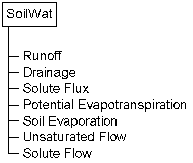
Figure 1. The subroutine structure of SoilWater.

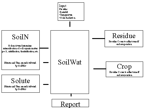
Figure 2. A diagram showing the communication between SoilWater and other APSIM modules.

Soil Moisture Properties

An example some soil properties used to configure the SoilWater soil water “bucket” is as follows.

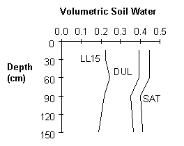
LL15 is the 15Bar lower limit of soil water content . It is approximately the driest water content achievable by plant extraction. This defines the “bottom of the bucket”.
DUL is the drained upper limit of soil water content . It is the content of water retained after gravitational flow. DUL is sometimes referred to as “Field Capacity”.
SAT is the Saturated water content . This defines the “top of the bucket”

Initial Soil Water

There are five ways to parameterise initial soil water in SoilWater.

These can also be specified in the Manager module sections using the ‘set’ command
e.g

SoilWater set insoil = 0.5 ()

1. Initial Soil Water as User Specified Soil Water Content

The user can initialise soil water content to any initial volumetric soil water content for each layer.
This can be done by setting the soil water parameter (sw) for each layer to a value between SAT and LL15.
To use this option the insoil parameter must be set to > 1.

2. Initial Soil Water as a Fraction of Available Soil Water distributed evenly down the profile

Initial soil water can be set to a fraction of the maximum available soil water in each layer.
Setting the insoil parameter to a fraction (0 = LL15, 1 = DUL) initialises the soil water parameter (initial sw values are ignored) to this fraction for each layer.

ie. If 0.0 <= Insoil <= 1.0, then
in each layer
Soil water (sw) = LL15 + ((DUL-LL15) x Insoil)

3. Initial Soil Water as a Fraction of Available Soil Water filling the profile from the top.

Initial soil water can be set to a fraction of the maximum extractable soil water in the whole profile.
The profile is filled from the top down until the fraction is reached. Setting the profile_fesw parameter to a fraction of total extractable soil water initialises the soil water for layers starting at the top of the profile to DUL, until the fraction is reached.
The remaining layers are set to LL15. This parameter is exclusive of the others.

eg. If
the soil profile has layers of 150, 150, 300 and 300 mm,
giving a total profile depth of 900 mm
with corresponding DUL of 67.5, 67.5, 135, 120 mm and
corresponding LL15 of 34.5, 34.5, 72, 75 mm giving
ESW of 33, 33, 63, 45 mm with a
Total ESW in the profile of 174 mm.
And
profile_fesw = 0.5,
Then
The ESW of each layer is set to 33, 33, 21, 0 mm giving
A total of 87 mm in the profile.

4. Initial Soil Water as a depth of available Soil Water from the top of the profile.

Initial soil water can be set to a depth of available soil water in the whole profile.
The profile is filled from the top down until the soilwater depth is reached.
Setting the profile_esw_depth parameter to a total available soil water initialises the soil water for layers starting at the top of the profile to DUL, until the amount of water is reached.
The remaining layers are set to LL15. This parameter is exclusive of the others.

eg. Using the soil parameters of the previous example and
profile_esw_depth = 87mm,
Then
The ESW of each layer is set to 33, 33, 21, 0 mm.

5. Initial Soil Water as a depth of wet soil, filled to field capacity.

Initial soil water can be set to a depth of wet soil.
The profile is filled from the top down until the soil depth is reached.
Setting the wet_soil_depth parameter to a depth of soil filled to field capacity (DUL) initialises the soil water for layers starting at the top of the profile to DUL, until the soil depth is reached.
The remaining layers are set to LL15. This parameter is exclusive of the others.

e.g. Using the soil parameters of the previous example and
wet_soil_depth = 400 mm,
Then
The ESW of each layer is set to 33, 33, 21, 0 mm giving
A total of 87 mm in the profile.

Runoff

Runoff from rainfall is calculated using the USDA-Soil Conservation Service procedure known as the curve number technique.
The procedure uses total precipitation from one or more storms occurring on a given day to estimate runoff.
The relation excludes duration of rainfall as an explicit variable, and so rainfall intensity is ignored.
When irrigation is applied it is assumed to be at low intensity and therefore no runoff is calculated.

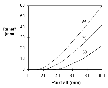
Runoff response curves (ie runoff as a function of total daily rainfall) are specified by numbers from 0 (no runoff) to 100 (all runoff).
Response curves for three runoff curve numbers for rainfall varying between 0 and 100 mm per day

The user supplies a curve number for average antecedent rainfall conditions (CN2Bare).
From this value the wet (high runoff potential) response curve and the dry (low runoff potential) response curve are calculated.
The SoilWater module will then use the family of curves between these two extremes for calculation of runoff depending on the daily moisture status of the soil.
The effect of soil moisture on runoff is confined to the effective hydraulic depth as specified in the module’s ini file and is calculated to give extra weighting to layers closer to the soil surface.

Runoff response curve for average antecedent rainfall condition curve number (CN2) of 75 for a range of soil moisture conditions
(0 – dry, 1 – wet).

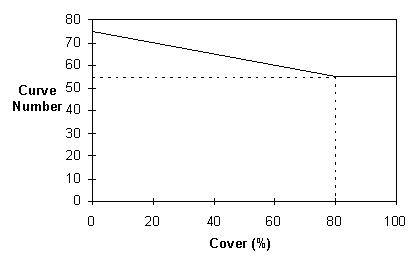
Residue cover effect on runoff curve number where bare soil curve number is 75 and total reduction in curve number is 20 at 80% cover.

Surface residues inhibit the transport of water across the soil surface during runoff events and so different families of response curves are used according to the amount of crop and residue cover. The extent of the effect on runoff is specified by:
a threshold surface cover (CNCov), above which there is no effect,
and the corresponding curve number reduction (CNRed).

Tillage of the soil surface also reduces runoff potential, and a similar modification of Curve Number is used to represent this process.
A tillage event is directed to the module, specifying cn_red, the CN reduction, and cn_rain, the rainfall amount required to remove the tillage roughness.
CN2 is immediately reduced and increases linearly with cumulative rain, ie. roughness is smoothed out by rain.

The effect of these processes is seen in the daily output variable CN2_new – the curve number used to calculate runoff on any particular day.

Evaporation

Soil evaporation is assumed to take place in two stages: the constant and the falling rate stages.

In the first stage the soil is sufficiently wet for water to be transported to the surface at a rate at least equal to the potential evaporation rate.
Potential evapotranspiration is calculated using an equilibrium evaporation concept as modified by Priestly and Taylor(1972).

Once the water content of the soil has decreased below a threshold value the rate of supply from the soil will be less than potential evaporation (second stage evaporation).
These behaviors are described in SoilWater through the use of two parameters: U and cona.

The parameter U (as from CERES) represents the amount of cumulative evaporation before soil supply decreases below atmospheric demand.

The rate of soil evaporation during the second stage is specified as a function of time since the end of first stage evaporation.

The parameter Cona (from PERFECT) specifies the change in cumulative second stage evaporation against the square root of time.

ie. E_s = cona t^1/2

Water lost by evaporation is removed from the surface layer of the soil profile thus this layer can dry below the wilting point or lower limit (LL) to a specified air-dry water content (air_dry).

SoilWater uses two parameters, U and CONA, to specify soil evaporation.
U(as in CERES) is the amount of cumulative evaporation, since soil wetting, before soil supply becomes limiting.
Subsequently soil evaporation is a fraction of the square root of time since the end of first stage evaporation, using the regression coefficient CONA ( from PERFECT).

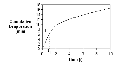
Cumulative Soil Evaporation through time for U = 6 mm and CONA = 3.5.

For t <= t₁
E_s = E_os

For t > t₁

Saturated Water Flow (between SAT and DUL)

When water content in any layer is below SAT but above DUL, a fraction of the water drains to the next deepest layer each day.

Flux = SWCON x (SW – DUL)

Infiltration or water movement into any layer that exceeds the saturation capacity of the layer automatically cascades to the next layer.

Unsaturated Water Flow (below DUL)

For water contents below DUL, movement depends upon the water content gradient between adjacent layers and the diffusivity,
which is a function of the average water contents of the two layers.

Unsaturated flow may occur both towards the surface and downwards, but cannot move water out of the bottom of the deepest layer in the profile.
Flow between adjacent layers ceases at a soil water gradient (gravity_gradient) specified in the SoilWater ini file.

The diffusivity is defined by two parameters set by the user (diffus_const, diffus_slope) in the SoilWater parameter set
(Default values, from CERES, are 88 and 35.4, but 40 and 16 have been found to be more appropriate for describing water movement in cracking clay soils).

Diffusivity = diffus_const x exp (diffus_slope x thet_av)

where,
thet_av is the average of SW – LL15 across the two layers.
Flow = Diffusivity x Volumetric Soil Water Gradient

Solute Movement

SoilWater can move any solute within the APSIM simulation.
Solutes are defined to be either mobile or immobile, according to specifications in the SoilWater module’s ini file.

The saturated and unsaturated flows of soil water are used to calculate the redistribution of solutes throughout the soil using a “mixing” algorithm which assumes that all water and solute entering or leaving a layer is completely mixed.
This means that solute movement can simply be calculated as the product of the water flow and the solute concentration in that water.

Fluxes of solutes are associated with both saturated and unsaturated water fluxes.
In both cases a simple mixing algorithm is used whereby incoming water and solute is fully mixed with that already present in any layer to obtain concentrations for solutes that are applied to the water leaving the layer.

Efficiency factors (flux_eff and flow_eff) are specified in the SoilWater ini file to adjust the effectiveness of mixing for either saturated or unsaturated flows.

Leaching

The amount of solute dissolved in water can move to the layer below. This is considered by the model to be leaching.
Individual solutes leached from each layer can be tracked by reporting the solute leaving the layer.
An example may include reporting no3_leach(7).
If there are 7 layers defined in the soil profile then this variable will represent the leaching of no3 out of the root zone.

Solutes in Rainfall

Solutes can be applied to the soil via rainfall using the optional parameter ‘rainfall_XXX_conc’ in parts per million,
where ‘XXX’ is the solute name.

As many solutes as desired can be applied in this way, however any solutes used must first be initialised in the system with the SOLUTE module.

Above Saturation Flow (above SAT)

When the soil water rises above Saturation there are two different parameters that can be specified: MWCON or KS.
Both of these are layered values, so you need to enter a value for each layer in the soil.

MWCON allows you to specify either 1 or 0 for each layer in the soil.

A value of 1 means that all water above saturation for that layer immediately flows straight into the layer below.
If this layer below is filled above saturation by water coming in from above and MWCON for that layer is 1 then this water then flows to the next layer and so forth for each of the layers below.
Eventually water will run out of the bottom layer as drainage (report “drain” to see this).
This is the tipping or cascading part of the classical tipping bucket or cascading flow analogy.

A value of 0 means that all water above saturation is NOT allowed to flow into the layer below. ie it is an impermeable layer.
Water will then begin to backup.
Note that depending on how SWCON is set, water will still be able to be lost from the layer via the process of Saturated Flow (the flow that occurs between DUL and SAT).
If both MWCON and SWCON prevent the water from flowing out of the layer then the water will begin to back up and will either become a pond on the surface or a water table beneath the surface.

KS allows you to specify a number of millimeters per day that is allowed to drain from the layer when the the soil water is above saturation.
Once again depending upon how SWCON is set, Saturated Flow may still occur, and once again if soil water backs up a pond or water table is generated.

nb. If neither MWCON or KS is set, then an MWCON value of 1 for each layer is assumed. ie. any water above saturation flows straight into the layer below.
If both MWCON and KS are set, then KS overrides MWCON.

Surface Ponding and Water Table Functionality

Soilwat has the functionality of simulating an impermeable layer(s) within the soil profile, above which a water table may perch.
The impermeable layer(s) is specified by setting either MWCON or KS (as mentioned in the previous section).

If the water-table happens to reach the surface, then Soilwat also has the ability to simulate a surface-storage (or ‘ponding’) pool.
The surface-water storage capacity is specified by the parameter max_pond, the maximum available surface water storage.
This max_pond is applied to both runoff from rainfall events and also to runoff generated by water backing-up above an impermeable layer (mxcon or ks) below.
Any surface water backing-up over ‘max_pond’ is added to the runoff pool.

There is also an output value called “pond_evap” which tells you the evaporation from the pond. This is separate from es which does NOT include pond evaporation in it.

MWCON, KS and max_pond are all optional parameters and if not provided, they are set to defaults (0.0 for max_pond).

Here is an example of setting up a pond:

[black_earth.soilwat2.parameters]

!layer 1 2 3 4 5 6 7

dlayer = 150 150 300 300 300 300 300 ! layer thickness mm soil

bd = 1.30 1.30 1.29 1.31 1.35 1.36 1.36 ! bulk density gm dry soil/cc moist soil

sat = .500 .509 .510 .505 .490 .480 .480 ! saturation mm water/mm soil

dul = .450 .459 .45 .44 .42 .41 .41 ! drained upper limit mm water/mm soil

sw = .280 .364 .43 .43 .40 .41 .41 ! initial soil water mm water/mm soil

ll15 = .230 .240 .240 .250 .260 .270 .280 ! lower limit mm water/mm soil

air_dry = .10 .20 .20 .20 .20 .20 .20 ! air dry mm water/ mm soil

swcon = 0.02 0.02 0.02 0.02 0.02 0.02 0.02 ! drainage coefficient

mwcon = 1.0 0.0 1.0 1.0 1.0 1.0 1.0

max_pond = 15.0 ! maximum depth of surface storage

nb. The two lines,

mwcon = 1.0 0.0 1.0 1.0 1.0 1.0 1.0

max_pond = 15.0 ! maximum depth of surface storage

Note, in layer 2 of mwcon, mwcon is set to 0.0 not 1.0 like all the other layers and therefore this layer is impermeable to ‘cascading’ flow, hence water cascading down the soil profile will reach this layer and begin to back-up towards the surface. Drainage is still allowed through this layer unless ‘swcon’ is also set to zero.

If the impermeable layer is specified deep down in the soil, then the water table might not reach the surface and pond. The output variable ‘water_table’ reports the depth of the water-table below the surface as measured from the ground surface. If there is no water table, ‘water_table’ = 10000 by default.

NB. There is a Pond module in APSIM. This Pond module calculates all the solute and nitrogen effects of having a pond above your soil. It grows algae etc and modfies the chemical processes going on in the soil (The processes that normally occur in the Soil Nitrogen module SoilN). The ponding we are discussing here are just the parts that effect the water balance and hence are dealt with in this Soil Water module.

Runon, Lateral Inflow and Outflow on a layer basis

Runon Capability

Surface ‘runon’ can now be input from a data file.
Soilwat2 does a daily ‘get’ to retrieve this information from the input module.
From a user’s point of view this means that ‘runon’ can be provided on a daily basis from the met file or from a separate input file.

For example :
[runon.sparse.data]

runon = 0

allow_sparse_data = true

year day runon

() () (mm)

1988 1 20

1988 5 17

1988 6 22

1988 10 25

1988 11 22

Lateral Inflow Capability

Lateral Inflow can be input as a layer-based array via the same method as ‘runon’. The parameter name is ‘inflow_lat(layer)’.

For example:

[runon.sparse.data]

runon = 0

allow_sparse_data = true

year day runon inflow_lat(1) inflow_lat(2) inflow_lat(3)

() () (mm) (mm) (mm) (mm)

1988 1 20 1 2 2

1988 5 17 2 1 2

1988 6 22 0 0 0

1988 10 25 1 1 1

1988 11 22 1 2 2

Both ‘runon’ and ‘inflow_lat(layer)’ are optional inputs to the model.

NB. with Lateral Inflow it is assumed that ALL the water goes straight into the layer. Irrespective of the layers ability to hold it. It is like an irrigation. Klat has no effect and does not alter the amount of water coming into the layer. Klat only alters the amount of water flowing out of the layer

Lateral Outflow Capability

Lateral Outflow is the flow that occurs as a result of the soil water going above DUL and the soil being on a slope. So if there is no slope and the water goes above DUL there is no lateral outflow. KLAT is just the lateral resistance of the soil to this flow. It is a soil water conductivity.

The calculation of lateral outflow on a layer basis is now performed using the equation:

Lateral flow for a layer = Klat * d * s/(1+s^2)^0.5 * L/A * unit conversions.

Where:
Klat = lateral conductivity (mm/day)

d = depth of saturation in the layer (mm)= dlayer*(sw-dul)/(sat-dul) if sw > dul.
Note this allows lateral flow in any “saturated” layer, not just those inside a water table.

s = slope (m/m)
L= catchment discharge width. Basically, it’s the width of the downslope boundary of the catchment. (m)
A = catchment area. (m2)

An example of the new soilwat2 input parameters (optional – if not included, lateral outflow = zero) are :

[black_earth.soilwat2.parameters]

slope =0.1

discharge_width = 50

catchment_area = 1000

klat = 0.5

There is a new reportable variable called outflow_lat(layer). This can be summed by reporting outflow_lat().

NB. Lateral outflow only occurs when the soil water for the layer is above Drained Upper Limit (DUL). The above calculation involving klat, slope, discharge width, and catchment area is used to calculate the Lateral Outflow from each layer.

SoilWater Module Outputs

Name	Units	Description
Es	mm	Daily soil evaporation
Eo	mm	Daily potential evapotranspiration
Eos	mm	Daily potential soil evaporation
cn2_new		Daily value CN2 adjusted for surface cover
Runoff	mm	Daily runoff
Drain	mm	Daily drainage from bottom of soil profile
infiltration	mm	Daily infiltration across the soil surface
eff_rain	mm	Effective Rainfall (Rainfall – Runoff – Drainage).
salb		Bare soil albedo
bd	g/cm³	Bulk density of the soil for each layer
esw	mm	Extractable soil water in each layer (ie. sw_dep – ll15_dep)
sw_dep	mm	Amount of water in each layer
sw	mm³ /mm³	Volumetric water content in each layer
dlayer	mm	Thickness of each soil layer
ll15_dep	mm	Amount of water corresponding to a soil potential of 15 bar
ll15	mm³ /mm³	Volumetric water content for each layer corresponding to a soil potential of 15 bar
dul_dep	mm	Amount of water at drained upper limit for each soil layer
dul	mm³ /mm³	Volumetric water content at drained upper limit for each soil layer
sat_dep	mm	Amount of water in each layer at saturation
sat	mm³ /mm³	Volumetric water content at saturation for each soil layer
air_dry_dep	mm	Amount of water retained at air_dry for each layer
air_dry	mm³ /mm³	Volumetric water content for air dry soil in each layer
flux	mm	Saturated water flux from each layer to the layer below
flow	mm	Unsaturated water movement between layers (+ve up)
flow_nnnn	kg/ha	Amount of solute nnnn in saturated water movement from each layer to the layer below (where ‘nnnn’ is the name of the solute)(eg. flow_no3)
water_table	mm	Depth of the water table (10000 if no water table present)
pond	mm	Surface ponding
outflow_lat	mm	Lateral outflow from each layer

SoilWater module actions

Reset

The reset action can be invoked to reset the module to the state specified within the module’s input data, which includes the soil moisture characteristics, runoff and evaporation parameters and the initial soil water profile.

The Reset action is identical to the initialise action used by the simulation engine at the start of the simulation except that a description of the reinitialised state is not printed in the simulation summary file.

APSIM Manager Example:

[sample.manager.start_of_day]

! reinitialise residues at the beginning of each sowing window

If day = 100 then

SoilWater reset

endif

Initialise

The initialise action has now been replaced by the reset action (see above).

Summary Report

At initialisation, at series of tables and useful information is printed to the simulation summary file for perusal by the user. These tables can be printed to the summary file at any point during the simulation as a detailed record of the system state at a particular time.

APSIM Manager Example:

[sample.manager.start_of_day]

! Print out a summary of module state to the summary file

If day = 100 then

SoilWater sum_report

endif

References

Jones, C.A., and J.R. Kiniry. 1986. CERES-Maize: A simulation model of maize growth and development. Texas A&M University Press, College Station, Texas.
Littleboy, M., D.M. Silburn, D.M. Freebairn, D.R. Woodruff, G.L. Hammer, and J.K. Leslie. 1992. Impact of soil erosion on production in cropping systems. I. Development and validation of a simulation model. Aust. J. Soil Res. 30, 757-774.
Priestly, C.H.B., and Taylor, R.J. (1972) On the assessment of surface heat and evaporation using large-scale parameters. Monthly Weather Review. 100, 81
Ritchie, J.T. (1972) Model for predicting evaporation from a row crop with incomplete cover. Water Resources Research. 8 , 1204.
Soil Conservation Service (1972) National Engineering Handbook Section 4: Hydrology, Soil Conservation Service, USDA, Washington.